Microstrip bộ lọc cho các ứng dụng lò vi sóng RF (P6)
Bạn đang xem bản rút gọn của tài liệu. Xem và tải ngay bản đầy đủ của tài liệu tại đây (544.75 KB, 30 trang )
CHAPTER 6
Highpass and Bandstop Filters
In this chapter, we will discuss some typical microstrip highpass and bandstop fil-
ters. These include quasilumped element and optimum distributed highpass filters,
narrow-band and wide-band bandstop filters, as well as filters for RF chokes. De-
sign equations, tables, and examples are presented for easy reference.
6.1 HIGHPASS FILTERS
6.1.1 Quasilumped Highpass Filters
Highpass filters constructed from quasilumped elements may be desirable for many
applications, provided that these elements can achieve good approximation of de-
sired lumped elements over the entire operating frequency band. Care should be
taken when designing this type of filter because as the size of any quasilumped ele-
ment becomes comparable with the wavelength of an operating frequency, it no
longer behaves as a lumped element.
The simplest form of a highpass filter may just consist of a series capacitor,
which is often found in applications for direct current or dc block. For more selec-
tive highpass filters, more elements are required. This type of highpass filter can be
easily designed based on a lumped-element lowpass prototype such as one shown in
Figure 6.1(a), where g
i
denote the element values normalized by a terminating im-
pedance Z
0
and obtained at a lowpass cutoff frequency ⍀
c
. Following the discus-
sions in the Chapter 3, if we apply the frequency mapping
⍀ = – (6.1)
where ⍀ and
are the angular frequency variables of the lowpass and highpass fil-
ters respectively, and
c
is the cutoff frequency of the highpass filter. Any series in-
c
⍀
c
ᎏ
161
Microstrip Filters for RF/Microwave Applications. Jia-Sheng Hong, M. J. Lancaster
Copyright © 2001 John Wiley & Sons, Inc.
ISBNs: 0-471-38877-7 (Hardback); 0-471-22161-9 (Electronic)
ductive element in the lowpass prototype filter is transformed to a series capacitive
element in the highpass filter, with a capacitance
C
i
= (6.2)
Likewise, any shunt capacitive element in the lowpass prototype is transformed to a
shunt inductive element in the highpass filter, with an inductance
L
i
= (6.3)
Figure 6.1(b) illustrates such a lumped-element highpass filter resulting from the
transformations.
In order to demonstrate the technique for designing a quasilumped element high-
pass filter in microstrip, we will consider the design of a three-pole highpass mi-
crostrip filter with 0.1 dB passband ripple and a cutoff frequency f
c
= 1.5 GHz (
c
=
2
f
c
). The normalized element values of a corresponding Chebyshev lowpass proto-
type filter are g
0
= g
4
= 1.0, g
1
= g
3
= 1.0316, and g
2
= 1.1474 for ⍀
c
= 1. The high-
pass filter will operate between 50 ohm terminations so that Z
0
= 50 ohm. Using de-
sign equations (6.2) and (6.3), we find
Z
0
ᎏ
c
⍀
c
g
i
1
ᎏ
Z
0
c
⍀
c
g
i
162
HIGHPASS AND BANDSTOP FILTERS
g
0
()a
g
1
g
2
g
3
g
4
g
n-1
g
n
g
n+1
()b
L
n-1
C
n
L
4
C
3
L
2
C
1
Z
0
Z
n+1
FIGURE 6.1 (a) A lowpass prototype filter. (b) Highpass filter transformed from the lowpass
prototype.
(a)
(b)
C
1
= C
3
= = = 2.0571 × 10
–12
F
L
2
= = = 4.6236 × 10
–9
H
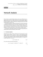
A possible realization of such a highpass filter in microstrip, using quasilumped el-
ements, is shown in Figure 6.2(a). Here it is seen that the series capacitors for C
1
and C
3
are realized by two identical interdigital capacitors, and the shunt inductor
for L
2
is realized by a short-circuited stub. The microstrip highpass filter is designed
on a commercial substrate (RT/D 5880) with a relative dielectric constant of 2.2 and
a thickness of 1.57 mm. In determining the dimensions of the interdigital capaci-
tors, such as the finger width, length and space, as well as the number of the fingers,
the closed-form design formulation for interdigital capacitors discussed in the
Chapter 4 may be used. Alternatively, full-wave EM simulations can be performed
to extract the two-port admittance parameters of an interdigital capacitor for differ-
ent dimensions. The desired dimensions are found such that the extracted admit-
tance parameter Y
12
= Y
21
at the cutoff frequency f
c
is equal to –j
c
C
1
. The interdig-
ital capacitor determined by this approach is comprised of 10 fingers, each of which
is 10 mm long and 0.3 mm wide, spaced by 0.2 mm with respect to the adjacent
ones. The dimensions of the short-circuited stub, namely the width W and length l,
can be estimated from
jZ
c
tan
l
= j
c
L
2
(6.4)
where Z
c
is the characteristic impedance of the stub line,
gc
is its guided wave-
length at the cutoff frequency f
c
, and both depend on the line width W on a sub-
strate. One might recognize that the term on the left-hand side of (6.4) is the input
impedance of a short-circuited transmission line. With a line width W = 2.0 mm on
the given substrate, it is found by using the microstrip design equations in Chapter 4
that Z
c
= 84.619 ohm and
gc
= 149.66 mm. Therefore, l = 11.327 mm is obtained
from (6.4), which is equivalent to an electrical length of 27.25° at 1.5 GHz. Al-
though the short-circuited stub of this length has a reactance matching to that of the
ideal inductor at the cutoff frequency, it will have about 36% higher reactance than
the idealized lumped-element design at 3 GHz. Generally speaking, to achieve a
good approximation of a lumped-element inductor over a wide frequency band, it is
essential to keep the length of a short-circuited stub as short as possible. This would
normally occur for a narrower line with higher characteristic impedance, which,
however, is restricted by fabrication tolerance and power-handling capability.
The final dimensions of the designed microstrip highpass filter as shown in Fig-
ure 6.2(a) were determined by EM simulation of the whole filter, taking into ac-
count the effects of discontinues and parasitical parameters. The EM simulated per-
formance of the final filter is plotted in Figure 6.2(b). It should be mentioned that
2
ᎏ
gc
50
ᎏᎏᎏ
2
× 1.5 × 10
9
× 1.1474
Z
0
ᎏ
c
⍀
c
g
2
1
ᎏᎏᎏᎏ
50 × 2
× 1.5 × 10
9
× 1.0316
1
ᎏᎏ
Z
0
c
⍀
c
g
1
6.1 HIGHPASS FILTERS
163
164
HIGHPASS AND BANDSTOP FILTERS
2.010.0
0.2
0.3
0.2
4.9
9.9
30
Via hole
grounding
25
Unit: mm
(a)
(b)
FIGURE 6.2 (a) A quasilumped highpass filter in microstrip on a substrate with a relative dielectric
constant of 2.2 and a thickness of 1.57 mm. (b) EM simulated performance of the quasilumped highpass
filter.
the interdigital capacitors start to resonate at about 3.7 GHz, which limits the usable
bandwidth. Reducing the size of the interdigital capacitors or replacing them with
appropriate microwave chip or beam lead capacitors can lead to an increase in the
bandwidth.
6.1.2 Optimum Distributed Highpass Filters
Highpass filters can also be constructed from distributed elements such as commen-
surate (equal electrical length) transmission-line elements. Since any commensurate
network exhibits periodic frequency response, the wide-band bandpass stub filters
discussed in Chapter 5 may be used as pseudohighpass filters as well, particularly
for wide-band applications, but they may not be optimum ones. This is because the
unit elements (connecting lines) in those filters are redundant, and their filtering
properties are not fully utilized. For this reason, we will discuss in this section an-
other type of distributed highpass filter [1].
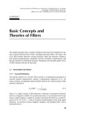
The type of filter to be discussed is shown in Figure 6.3(a), which consists of a
cascade of shunt short-circuited stubs of electrical length
c
at some specified fre-
quency f
c
(usually the cutoff frequency of high pass), separated by connecting lines
(unit elements) of electrical length 2
c
. Although the filter consists of only n stubs, it
has an insertion function of degree 2n – 1 in frequency so that its highpass response
has 2n – 1 ripples. This compares with n ripples for an n-stub bandpass (pseudo high-
pass) filter discussed in Chapter 5. Therefore, the stub filter of Figure 6.3(a) will have
a fast rate of cutoff, and may be argued to be optimum in this sense. Figure 6.3(b) il-
lustrates the typical transmission characteristics of this type of filter, where f is the
frequency variable and
is the electrical length, which is proportional to f, i.e.,
=
c
(6.5)
For highpass applications, the filter has a primary passband from
c
to
–
c
with a
cutoff at
c
. The harmonic passbands occur periodically, centered at
= 3
/2, 5
/2,
···, and separated by attenuation poles located at
=
, 2
, ···. The filtering
characteristics of the network in Figure 6.3(a) can be described by a transfer (inser-
tion) function
|S
21
(
)|
2
= (6.6)
where
is the passband ripple constant,
is the electrical length as defined in (6.5),
and F
N
is the filtering function given by
F
N
(
) = (6.7)
(1 +
͙
1
ෆ
–
ෆ
x
ෆ
c
2
ෆ
)T
2n–1
ᎏ
x
x
c
ᎏ
– (1 –
͙
1
ෆ
–
ෆ
x
ෆ
c
2
ෆ
)T
2n–3
ᎏ
x
x
c
ᎏ
ᎏᎏᎏᎏᎏ
2 cos
ᎏ
2
ᎏ
–
1
ᎏᎏ
1 +
2
F
N
2
(
)
f
ᎏ
f
c
6.1 HIGHPASS FILTERS
165
where n is the number of short-circuited stubs,
x = sin
–
, x
c
= sin
–
c
(6.8)
and T
n
(x) = cos(n cos
–1
x) is the Chebyshev function of the first kind of degree n.
Theoretically, this type of highpass filter can have an extremely wide primary
passband as
c
becomes very small, however, this may require unreasonably high
ᎏ
2
ᎏ
2
166
HIGHPASS AND BANDSTOP FILTERS
y
1
y
2
y
n-1
y
0
=1
2
θ
c
θ
c
y
n
y
1,2
y
n-1,n
Short-circuited stub
of electrical length
θ
c
y
0
=1
2
θ
c
(a)
(b)
FIGURE 6.3 (a) Optimum distributed highpass filter. (b) Typical filtering characteristics of the opti-
mum distributed highpass filter.
impedance levels for short-circuited stubs. Nevertheless, practical stub filter de-
signs will meet many wide-band applications. Table 6.1 tabulates some typical ele-
ment values of the network in Figure 6.3(a) for practical design of optimum high-
pass filters with two to six stubs and a passband ripple of 0.1 dB for
c
= 25°, 30°,
and 35°. Note that the tabulated elements are the normalized characteristic admit-
tances of transmission line elements, and for given terminating impedance Z
0
the
associated characteristic line impedances are determined by
Z
i
= Z
0
/y
i
(6.9)
Z
i,i+1
= Z
0
/y
i,i+1
Design Example
To demonstrate how to design this type of filter, let us consider the design of an op-
timum distributed highpass filter having a cutoff frequency f
c
= 1.5 GHz and a 0.1
dB ripple passband up to 6.5 GHz. Referring to Figure 6.3(b), the electrical length
c
can be found from
– 1
f
c
= 6.5
This gives
c
= 0.589 radians or
c
= 33.75°. Assume that the filter is designed with
six shorted-circuited stubs. From Table 6.1 we could choose the element values for
n = 6 and
c
= 30°, which will gives a wider passband, up to 7.5 GHz, because the
smaller the electrical length at the cutoff frequency, the wider the passband. Alter-
natively, we can find the element values for
c
= 33.75° by interpolation from the el-
ᎏ
c
6.1 HIGHPASS FILTERS
167
TABLE 6.1 Element values of optimum distributed highpass filters with 0.1 dB ripple
y
1
y
1,2
y
2
y
2,3
y
3
n
c
y
n
y
n–1,n
y
n–1
y
n–2,n–1
y
n–2
y
3,4
2 25° 0.15436 1.13482
30° 0.22070 1.11597
35° 0.30755 1.08967
3 25° 0.19690 1.12075 0.18176
30° 0.28620 1.09220 0.30726
35° 0.40104 1.05378 0.48294
4 25° 0.22441 1.11113 0.23732 1.10361
30° 0.32300 1.07842 0.39443 1.06488
35° 0.44670 1.03622 0.60527 1.01536
5 25° 0.24068 1.10540 0.27110 1.09317 0.29659
30° 0.34252 1.07119 0.43985 1.05095 0.48284
35° 0.46895 1.02790 0.66089 0.99884 0.72424
6 25° 0.25038 1.10199 0.29073 1.08725 0.33031 1.08302
30° 0.35346 1.06720 0.46383 1.04395 0.52615 1.03794
35° 0.48096 1.02354 0.68833 0.99126 0.77546 0.98381
ement values presented in the table. As an illustration, for n = 6 and
c
= 33.75°, the
element value y
1
is calculated as follows:
y
1
= 0.35346 + × 3.75 = 0.44909
In a similar way, the rest of element values are found to be
y
1,2
= 1.03446, y
2
= 0.63221, y
2,3
= 1.00443, y
3
= 0.71313, y
3,4
= 0.99734
These interpolated element values are well within one percent of directly synthe-
sized element values. The filter is supposed to be doubly terminated by Z
0
= 50
ohms. Using (6.9), the characteristic impedances for the line elements are Z
1
= Z
6
=
111.3 ohms, Z
2
= Z
5
= 79.1 ohms, Z
3
= Z
4
= 70.1 ohms, Z
1,2
= Z
5,6
= 48.3 ohms, Z
2,3
= Z
4,5
= 49.8 ohms, and Z
3,4
= 50.1 ohms.
The filter is realized in microstrip on a substrate with a relative dielectric con-
stant of 2.2 and a thickness of 1.57 mm. The initial dimensions of the filter can be
easily estimated by using the microstrip design equations discussed in Chapter 4 for
realizing these characteristic impedances and the required electrical lengths at the
cutoff frequency, namely,
c
= 33.75° for all the stubs and 2
c
= 67.5° for all the
connecting lines. The final filter design with all the determined dimensions is
shown in Figure 6.4(a), where the final dimensions have taken into account the ef-
fects of discontinues, and have been slightly modified to allow all the connecting
lines to have a 50 ohm characteristic impedance. The design is verified by full-wave
EM simulation. Figure 6.4(b) is the simulated performance of the filter; we can see
that the filter frequency response does show eleven or 2n – 1 ripples in the designed
passband, as would be expected for this type of optimum highpass filter with only
n = 6 stubs.
6.2 BANDSTOP FILTERS
6.2.1 Narrow-Band Bandstop Filters
Figure 6.5 shows two typical configurations for TEM or quasi-TEM narrow-band
bandstop filters. In Figure 6.5(a), a main transmission line is electrically coupled to
half-wavelength resonators, whereas in Figure 6.5(b), a main transmission line is
magnetically coupled to half-wavelength resonators in a hairpin shape. In either
case, the resonators are spaced a quarter guided wavelength apart. If desired, the
half-wavelength, open-circuited resonators may be replaced with short-circuited,
quarter-wavelength resonators having one end short-circuited.
A simple and general approach for design of narrow-band bandstop filters is
based on reactance/susceptance slope parameters of the resonators. To employ a
lowpass prototype, such as those discussed in Chapter 3, for bandstop filter design,
the transition from lowpass to bandstop characteristics can be effected by frequency
mapping
(0.48096 – 0.35346)
ᎏᎏᎏ
5
168
HIGHPASS AND BANDSTOP FILTERS
⍀ =
0
=
͙
ෆ
1
ෆ
2
ෆ
(6.10)
FBW =
where ⍀ is the normalized frequency variable of a lowpass prototype, ⍀
c
is its cut-
off, and
0
and FBW are the midband frequency and fractional bandwidth of the
2
–
1
ᎏ
0
⍀
c
FBW
ᎏᎏ
(
/
0
–
0
/
)
6.2 BANDSTOP FILTERS
169
150
30
Via hole
grounding
0.9
2.0 2.8
13.9
13.5
13.2
23.8 23.0 22.7
4.9
Unit: mm
(a)
(b)
FIGURE 6.4 (a) A microstrip optimum highpass filter on a substrate with a relative dielectric constant
of 2.2 and a thickness of 1.57 mm. (b) EM simulated performance of the microstrip optimum highpass
filter.
bandstop filter. The band-edge frequencies
1
and
2
are indicated in Figure 6.6.
Two equivalent circuits for the bandstop filters of Figure 6.5 can then be obtained as
depicted in Figure 6.7, where Z
0
and Y
0
denote the terminating impedance and ad-
mittance, Z
U
and Y
U
are the characteristic impedance and admittance of immittance
inverters, and all the circuit parameters including inductances L
i
and capacitances C
i
can be defined in terms of lowpass prototype elements [2]. For the circuit in Figure
6.7(a):
ᎏ
Z
Z
U
0
ᎏ
2
=
ᎏ
g
0
g
1
n+1
ᎏ
(6.11a)
x
i
=
0
L
i
=
ᎏ
0
1
C
i
ᎏ
= Z
0
ᎏ
Z
Z
U
0
ᎏ
2
for i = 1 to n
g
0
ᎏᎏ
g
i
⍀
c
FBW
170
HIGHPASS AND BANDSTOP FILTERS
FIGURE 6.5 TEM or quasi-TEM narrow-band bandstop with (a) electric couplings and (b) magnetic
couplings.
(b)
(a)
6.2 BANDSTOP FILTERS
171
FIGURE 6.6 Bandstop filter characteristics defining midband frequency and band-edge frequencies.
(a) Chebyshev characteristic. (b) Butterworth characteristic.
FIGURE 6.7 Equivalent circuits of bandstop filters with (a) shunt series-resonant branches and (b) se-
ries parallel-resonant branches.
()b
L
n
C
n
L
3
C
3
Y
0
Y
0
L
2
C
2
90
o
Y
U
L
1
C
1
90
o
Y
U
L
n
C
n
L
3
C
3
Z
0
Z
0
()a
L
2
C
2
90
o
Z
U
90
o
Z
U
L
1
C
1
where g
i
are the element values of lowpass prototype, and x
i
are the reactance slope
parameters of shunt series resonators. For series branches in Figure 6.7(b):
ᎏ
Y
Y
U
0
ᎏ
2
=
ᎏ
g
0
g
1
n+1
ᎏ
(6.11b)
b
i
=
0
C
i
=
ᎏ
1
0
L
i
ᎏ
= Y
0
ᎏ
Y
Y
U
0
ᎏ
2
ᎏ
g
i
⍀
c
g
F
0
BW
ᎏ
for i = 1 to n
where b
i
are the susceptance slope parameters of series parallel resonators.
It is obvious that for a chosen lowpass prototype, with known element values, the
desired reactance/susceptance slope parameters can easily be determined using
(6.11). The next step is to design microwave bandstop resonators such as those in
Figure 6.5 so as to have prescribed slope parameters. A practical and general tech-
nique that allows one to extract slope parameters of microwave bandstop resonators
using EM simulations or experiments is discussed next.
Consider a two-port network with a single shunt branch of Z = j
L + 1/(j
C),
such as the one in Figure 6.7(a). The shunt branch resonates at
0
= 1/
͙
L
ෆ
C
ෆ
and has
a reactance slope x =
0
L. The transmission parameter for this two-port network
terminated with Z
0
is given by
S
21
= (6.12)
Let
=
0
+ ⌬
. In narrow-band cases, ⌬
Ӷ
0
, and thus the shunt impedance
may be approximated by
Z Ϸ j
0
L
(6.13)
in which the approximation (
/
0
–
0
/
) Ϸ 2⌬
/
0
has been made. By substitu-
tion, we can obtain from (6.12)
|S
21
| = (6.14)
This is at resonance when
=
0
or ⌬
= 0, |S
21
| = 0 because the resonant shunt
branch shorts out the transmission and causes an attenuation pole. When the fre-
quency shifts such that
= ±1 (6.15)
the value of |S
21
| has risen to 0.707 or –3 dB. From (6.15), a 3 dB bandwidth can be
defined by
0
ᎏ
⌬
±
1
ᎏ
4(x/Z
0
)
1
ᎏᎏᎏ
Ί
1
+
΄
ᎏ
4
(x
1
/Z
0
)
ᎏ
ᎏ
⌬
0
ᎏ
΅
2
2⌬
ᎏ
0
1
ᎏ
1 +
ᎏ
2
Z
Z
0
ᎏ
172
HIGHPASS AND BANDSTOP FILTERS