Modeling, Measurement and Control P26

26

Mobile Robotic Systems

26.1 Introduction
26.2 Fundamental Issues

Definition of a Mobile Robot • Stanford Cart •
Intelligent Vehicle for Lunar/Martian Robotic
Missions • Mobile Robots — Nonholonomic Systems

26.3 Dynamics of Mobile Robots
26.4 Control of Mobile Robots

26.1 Introduction

This subsection is devoted to modeling and control of mobile robotic systems. Because a mobile
robot can be used for exploration of unknown environments due to its partial or complete autonomy
is of fundamental importance. It can be equipped with one or more manipulators for performing
mission-specific operations. Thus, mobile robots are very attractive engineering systems, not only
because of many interesting theoretical aspects concerning intelligent behavior and autonomy, but
also because of applicability in many human activities. Attractiveness from the theoretical point of
view is evident because no firm fundamental theory covering intelligent control independent of
human assistance exists. Also, because wheeled or tracked mobile robots are nonholonomic mechan-
ical systems, they are attractive for nonlinear control and modeling research. In Section 26.2 of
this chapter, fundamental issues are explained regarding nonholonomic systems and how they differ
from holonomic ones. Although we will focus attention mostly on wheeled mobile robots, those
equipped with tracks and those that rely on legged locomotion systems are addressed as well. The

term “mobility” is addressed from the standpoint of wheeled and tracked platform geometry.
Examples provided are also showing how different platforms have been built in practice.
Section 26.3 covers dynamics of mobile robots. Models range from very complex ones that
include dynamics of deformable bodies to relatively simple models mostly used to facilitate
development of control algorithms. The discussion concludes with some model transformations
that help obtain relatively simple models.
The next section is devoted to control issues from the standpoint of both linear and nonlinear
control theories. We explain the difference between controllability in the linear system theory and
controllability of mobile robots, having in mind that a mobile robot is a nonlinear system.

26.2 Fundamental Issues

26.2.1 Definition of a Mobile Robot

A definition of a mobile robotic system does not exist. The International Standards Organization
(ISO), has defined an industrial robot as:

Nenad M. Kircanski

University of Toronto

8596Ch26Frame Page 707 Friday, November 9, 2001 6:25 PM
© 2002 by CRC Press LLC


Definition 1:

An

industrial robot

is an automatic, servo-controlled, freely programmable, multi-
purpose

manipulator

, with several axes, for the handling of workpieces, tools, or special devices.
Variably programmed operation make possible the execution of a multiplicity of tasks.
This definition clearly indicates that the term “industrial robot” is linked to a “manipulator,”
meaning that such a mechanical system is attached to a base. Typically, the base is fixed with
respect to a ground or single-degree-of-freedom platform mounted on rails. We also observe that
an industrial robot must have a programmable control system so that the same robot can be used
for different tasks.
A mobile robot has two essential features that are not covered by this definition. The first is
obviously mobility, and the second is autonomy. A minimum requirement for a mobile robot is to
be capable of traversing over flat horizontal surfaces. Given a point

A

on such a surface

S

, where
the robot is positioned at a time instant

t

, the mobile robot must be capable of reaching any other
point

B

at a certain distance

d

<

∞

from

A

, in a finite time

T

. Here, we should clarify the meaning
of the term “position.” Let us assume that a coordinate frame

Oxyz

is attached to the surface so
that

O

belongs to the surface, while the

z

-axis is normal to the surface (Figure 26.1). Clearly, the
position of any point on the surface is defined by coordinates (

x

,

y

). But, the position of the robot
is actually defined by the coordinates (

x

,

y,



φ

), where

φ

defines the orientation of the chassis with
respect to the

x

axis. Of course the orientation can be defined in many different ways (for example,
with respect to

y

or any other axis in the plane surface). So, mobility means that the robot is capable
of traversing from the position (

x

A

,

y

A

,



φ

A

) to (

x

B

,

y

B

,



φ

B

) in a finite time interval

T

.
Mobility, as discussed above, is limited in terms of the system’s ability to traverse different
surfaces. The simplest case is a flat horizontal surface

z

= constant. Most 4-wheel mobile robots
are designed for such terrains. In the case of a smooth surface

z

=

f

(

x

,

y

), where

f

is an arbitrary
continuous function of

x

and

y

, the ability of a wheeled robot to reach any desired point

B

from a
point

A

on the surface depends upon (1) the ability of the robot to produce enough driving force
to compensate for gravity force while moving toward the goal point; and (2) the presence of
sufficient friction forces between the wheels and the ground to prevent continuous slippage. Notice
also that there is no uniquely defined path between the points

A

and

B

, and the robot may be
incapable of traversing some trajectories, but still capable of reaching point

B

provided the trajectory
is conveniently selected.
In discussions related to mobility a fundamental question concerns climbing and descending

stairs, over-crossing channels, etc. Previously we have implicitly assumed that the function

f

is
differentiable with respect to

x

and

y

. If this does not hold, as is true for a staircase, mobility can
be achieved with tracks or legs. Robots with legs are called “legged-locomotion robots.” Such
robots are rarely used in practice due to the complexity (and thus reliability and cost) of the
locomotion subsystem. Tracked robots are usually six-wheel robots with a set of two tracks mounted
on three wheels on the left and three wheels on the right side of the chassis. Each track has a tread

FIGURE 26.1

Definition of coordinates.


8596Ch26Frame Page 708 Friday, November 9, 2001 6:25 PM
© 2002 by CRC Press LLC


that engages with the edge of the first stair of a staircase. Such engagement allows for lifting the
front side of the chassis while the back side remains on the ground. In this phase of climbing, the

vehicle tilts backward while moving forward and finally reaches an inclination angle equal to that
of the staircase. The tread on the tracks engages with several stairs simultaneously, allowing the
robot to move forward.
In the second part of this section, the mobility will be highlighted from the standpoint of
nonholonomic constraints. We explain why a manipulator is a holonomic and why a mobile robot
is a nonholonomic system. Prior to that, though, we attempt to define a mobile robot. As mentioned
at the beginning of this section, the second essential feature of a mobile robot is autonomy. We
know that vehicles have been used as a means of transportation for centuries, but vehicles were
never referred to as “mobile robots” before, because the fundamental feature of a robot is to perform
a task without human assistance. In an industrial, well-structured environment it is not difficult to
program a robot manipulator to perform a task. On the other hand, the term “mobile robot” does
not necessarily correlate to an industrial environment, but a natural or urban environment. Industrial
mobile robots are called automatic guided vehicles (AGVs). AGVs are mobile platforms typically
guided by an electromagnetic source (a set of wires) placed permanently under the floor cover.
Tracking of the guidelines is realized through a simple feedback/feedforward control. Thus, an
AGV is not referred to as a mobile robot because it is not an autonomous system.
An autonomous system must be capable of performing a task without human assistance and
without relying on an electronic guidance system. It must have sensors to identify environmental
changes, and it must incorporate planning and navigation features to accomplish a task. More details
about these features are given in later sections, but now we provide an example of a simple mobile
robot currently used in urban environments: a vacuum-cleaning mobile robot. Such commercially
available robots have an ultrasonic-based range-finder mounted on a pan-and-tilt unit. This unit is
located on the front end of the chassis and constantly rotates left-and-right and up-and-down
independently of the speed of the vehicle. The range-finder is an ultrasonic transceiver/receiver
sensor mounted on the unit end-point. The echoes are processed by an on-board computer to identify
obstacles around the robot. A planner is a software module that describes the “desired path” so
that cleaning is performed uniformly all over the floor surface. The navigator is the software module
that provides changes in desired trajectories in accordance with the obstacles/walls located by the
sensorial system. Such a robot will automatically slow down and avoid a collision should another
vehicle or a human traverse its trajectory. Clearly, autonomy is not necessarily correlated to artificial

intelligence. “Intelligent control” can be a feature of a mobile robot, but it is not a must in practice.
Based on the previous discussion we can define a mobile robot as follows:

Definition 2:

A

mobile robot

is an autonomous system capable of traversing a terrain with natural
or artificial obstacles. Its chassis is equipped with wheels/tracks or legs, and, possibly, a manipulator
setup mounted on the chassis for handling of work pieces, tools, or special devices. Various
preplanned operations are executed based on a preprogrammed navigation strategy taking into
account the current status of the environment.
Although this is not an official definition proposed by ISO, it contains all the essential features
of a mobile robot. According to this definition, an AGV is not a mobile robot because it lacks
autonomy and the freedom to traverse a terrain (it is basically a single-degree-of-freedom moving
platform along a built-in guide path). Similarly, “teleoperators,” used in the nuclear industry for
decades, are not mobile robots for the same reason: a human operator has full control over the
vehicle. A teleoperator looks like a mobile robot because it has a chassis and a manipulator arm
on top of it, but its on-board computer is programmed to follow the remote operator’s commands.
An example of a real mobile robot is the four-wheel Stanford Cart built in the late seventies.

1

This
relatively simple robot, as well as some advanced ones, including an intelligent robotic vehicle
recently developed for Lunar/Martian robotic missions, are described in the text to follow.

8596Ch26Frame Page 709 Friday, November 9, 2001 6:25 PM

© 2002 by CRC Press LLC


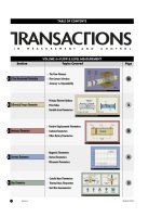
26.2.2 Stanford Cart

The cart was developed at the Stanford Artificial Intelligence Laboratory as a research setup for
Ph.D. students (Figure 26.2). The robot was equipped with an on-board TV system and a computer
dedicated to image processing and driving the vehicle through obstacle-cluttered spaces. The system
gained its knowledge entirely from images. Objects were located in three dimensions, and a model
of the environment was built with information gained while the vehicle was traversing a terrain.
The system was unreliable for long runs and very slow (1 m in 10 to 15 min).
The operation would start at a certain point on a flat horizontal surface (flat floor) cluttered with
obstacles. The camera was mounted on a sliding unit (50-cm track on top of the chassis) so that
it was able to move sideways while keeping the line-of-sight forward. Such sidewise movements
allowed the collection of several images of the same scene with a fixed lateral offset. By correlating
those images the control system was able to identify locations of obstacles in the camera’s field of
vision. Control was simplified because these images were collected while the cart was inactive.
After identifying the location of obstacles as simple fuzzy ellipsoids projected on the floor surface,
the vehicle itself was modeled as a fuzzy ellipsoid projected on the same surface.
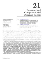
Based on the environment model a Path Planner was used to determine the shortest possible path
to the goal-point. This program was capable of finding the path that was either a straight segment
between the end and initial points, or a set of tangential segments and arcs along the ellipses
(Figure 26.3). To simplify the algorithm, the ellipses were actually approximated by circles.
The navigation module was very primitive because the chart motor control lacked feedback.
Thus, the vehicle was moved roughly in a certain direction by activating, driving, and steering
motors for a brief time. After moving the vehicle for about 1 m, the whole procedure was repeated.
Although the whole process was extremely slow (roughly 4 to 6 m/h), and vehicle control very
primitive, this was one of the first platforms that had all features needed for a robot to be regarded
as a real mobile robot. It was autonomous and adaptable to environmental variations.

26.2.3 Intelligent Vehicle for Lunar/Martian Robotic Missions

In contrast to the Stanford Cart built as a students’ experimental setup in the late 1970s, the
intelligent robotic vehicle system (IRVS) was developed by the UA/NASA Space Engineering
Research Center in the early 1990s.

2

This robot was developed to facilitate

in situ

exploration
missions on the lunar/Martian surface. The system was designed to determine (1) site topography
using two high-resolution CCD cameras and stereo-photogrammetry techniques; (2) surface mineral
composition using two spectrometers, an oven soil heater, and a gas analyzer; and (3) regolith
depths using sonar sounders. The primary goal of such missions was to provide accurate information
that incorporates

in situ

resource utilization on the suitability of a site to become a lunar/Martian
outpost. Such a lunar base would be built using locally available construction materials (rocks and

FIGURE 26.2

The Stanford Cart.

8596Ch26Frame Page 710 Friday, November 9, 2001 6:25 PM
© 2002 by CRC Press LLC

minerals). The base would allow building plants for the production of oxygen and hydrogen for
rocket fuel, helium for nuclear energy, and some metals. These materials would be used for building
space stations with a cost far lower than the cost of transporting them from Earth.
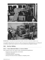
The IRVS consists of a mobile platform, a manipulator arm, and a set of mission sensors. The
most important requirement for the platform is exceptionally high payload-to-mass ratio. This was
achieved by using a Stewart platform system developed by the U.S. National Institute of Standards
and Technology (Figure 26.4). The structure consists of (1) an octahedral frame constructed of thin
walled aluminum tubing, (2) three wheel assemblies (two of them have speed/skid steering control,
while the third is a single free wheel), and (3) a work platform suspended by six cables arranged
as a Stewart platform. The system is equipped with two high-resolution cameras with power zoom,
auto iris, and focus capabilities mounted on a pan/tilt unit at the top of the octahedral frame.
Ultrasonic ranging sensors were added for detects objects within a range of 0.2 to 12 m with a
field of view of 6°. The system is also equipped with roll-and-pitch sensors that are used for
controlling the six cables so that the work platform is always horizontal.

FIGURE 26.3

Path Planning results for two distinct scenarios: (a) a straight line segment exists between the initial
and final point,

A

and

B

; and (b) a path consists of a set of straight segments tangential to augmented obstacles,
and arcs along the obstacle boundaries that are optimal in terms of its length.

FIGURE 26.4

IRVS mobile robot.

8596Ch26Frame Page 711 Friday, November 9, 2001 6:25 PM
© 2002 by CRC Press LLC


The IRVS control system is nontraditional, i.e., it is not based on sensing, planning, and executing
control levels. It consists of a number of behavior programs organized in control levels:

organiza-
tion

,

coordination,

and

execution

. The organization level consists of four behavior programs: (1)

site-navigator

, (2)

alternative sample collection point

(SCP)

selector

, (3) SCP

recorder

, and (4)
SCP

organizer

.
The site-navigator uses a potential field method to calculate the vehicle’s trajectory to the next
SCP based on vision and range measurements. The alternative SCP selector picks an alternative
SCP when a scheduled SCP cannot be reached due to obstacles/craters. The SCP recorder marks
the points already visited so that the vehicle cannot sample a SCP twice. The SCP organizer
generates a sequence of manipulator and instrument deployment tasks when the robot arrives at a
SCP.
The coordination level contains

task-dispatcher

and

behavior arbitrator

programs. The task-

dispatcher program analyzes the tasks submitted from the organization level, and activates the
behaviors (tasks at the execution level) needed for successful completion of the task’s requirements.
It also implements a set of failure procedures when a given task cannot be executed because of
possible failure (unstable vehicle, etc.). The behavior arbitrator assigns priorities to behaviors so
that only the highest-priority behavior will be executed when two or more are simultaneously
activated.
Execution level behaviors include the following tasks: obstacle-avoider, open-terrain explorer,
etc. Obstacle avoiders are activated when an ultrasonic sensor measurement indicates the presence
of an obstacle. Then, the site-navigator behavior is immediately suppressed due to its lower
priority than that of the obstacle avoider. The purpose of the open-terrain explorer is to monitor
obstacles in an open terrain situation and prevent the vehicle from becoming trapped among
obstacles.
Clearly, IRVS control architecture is similar to that of a multitasking real-time kernel. Control
is divided over a large number of tasks (called behaviors). The tasks are activated from a control
kernel so that the highest-priority one will run first. The control algorithm implemented within a
task (behavior) is usually simple and easy to test. The interdependencies among the control laws
are implemented within the task’s intercommunication network. Message envelopes, circular buff-
ers, semaphores, sockets, and other communication means are used for this purpose. Such control
architecture has “fine-granularity” so that elementary control tasks are simple. Still, the overall
control architecture is very complex and difficult for theoretical analysis.

26.2.4 Mobile Robots — Nonholonomic Systems

The Stanford Cart and IRVS are just two examples of mobile robots. From these examples we see
that mobile platforms can differ in many aspects including geometry, number of wheels, frame
structure, etc. From a mechanical point of view there is a common feature to all systems: they are
nonholonomic systems. In this section we explain exactly what that means.
Recall that the dynamic model of a manipulator with

n

degrees of freedom is described by
(26.1)
where

H

(

q

) is the

n



×



n

inertia matrix; is the

n

-vector due to gravity, centrifugal, and Coriolis
forces;

τ

is the

k

-dimensional input vector (note that not all joints are necessarily equipped with
actuators);

J

(

q

) is a

m



×



n

Jacobian matrix; and

f

is the

m

vector of constraint forces. The constraint
equation generally has the form
(26.2)
Hqq hqq J q f
T
() (,) ()
.. .
+=−τ
hqq(, )
.
Cqq(,)
.
= 0

8596Ch26Frame Page 712 Friday, November 9, 2001 6:25 PM
© 2002 by CRC Press LLC


where

C

is an

m

vector. Note that the constraint Equation (26.2) involves both the generalized
coordinates and its derivatives. In other words, the constraints may have their origins in the system’s
geometry and/or kinematics.
A typical system with geometric constraints is the robot shown in Figure 26.5. It has six joints
(generalized coordinates), but only three degrees of freedom. Assuming that the closed loop chain
ABCD is a parallelogram (Figure 26.5), the constraint equations are
In this case the constraint equations have form

C

i

(

q

) = 0. Such constraints, or those that can be
integrated into this form, are called

holonomic constraints

.
Another example is a four-degrees-of-freedom manipulator in contact with the bottom surface
with an end-effector normal to the surface (Figure 26.6). Assuming that the link lengths are equal
we obtain the following constraints:

FIGURE 26.5

A manipulator with a closed-loop chain within its structure.

FIGURE 26.6

A manipulator in contact with the environment.
qq
qq
qq
32
42
5
2
0
0
0
+−=
−=
+−=
π
π
qq
qq
qqqq
14
23
1234
0
0
30
−=
−=

+++− =π

8596Ch26Frame Page 713 Friday, November 9, 2001 6:25 PM
© 2002 by CRC Press LLC


A typical system with both holonomic and nonholonomic constraints is a two-wheel platform
supported by two additional free wheels in points

P

1

and

P

2

(Figure 26.7). Because the vehicle
consists of three rigid bodies (a chassis and two wheels), we can select the following five generalized
coordinates:

x

and

y

coordinates of the central point

C; an angle
φ
between the longitudinal axis
of the chassis (x
b
) and the x-axis of the reference frame; and
θ
L
and
θ
R
, the angular displacements
of the left and right wheel, respectively. We assume that the wheels are independently driven and
parallel to each other. The distance between the wheels is l.
The constraint equations can be derived from the fact that the vehicle velocity vector v is always
along the axis x
b
. In other words, the lateral component of the velocity vector (the one that is normal
to the wheels) is zero. From Figure 26.7 we observe that the unit vector along x
b
is ,
while the vector normal to direction of motion is
Because , and v⋅n = 0, we obtain the first constraint equation:
(26.3)
The other two constraint equations are obtained from the condition that the wheels roll, but do not
slip, over the ground surface:
where v
R
(v

L
) is the velocity of the platform at the points R (L) in Figure 26.7. Velocities and
are angular velocities of the right- and left-hand side wheel. The velocity vector in either of
these two points has two components: one due to the linear velocity of the chassis, and another
due to the rotation of the chassis. The first component is easily obtained as
(26.4)
from
(26.5)
(26.6)
FIGURE 26.7 A simple mobile platform.
x
b
T
= (cos sin )
φφ
x
b
T
= (cos sin )
φφ
v = (, )
..
xy
T
yx
..
cos sin
φφ
−=0
vr

vr
R
R
L
L
=
=
θ
θ
.
.
θ
.
R
θ
.
L
vx y=+
..
cos sin
φφ
xv
.
cos=
φ
yv
.
sin=
φ
8596Ch26Frame Page 714 Friday, November 9, 2001 6:25 PM

© 2002 by CRC Press LLC