Bài giảng giải tích hàm nhiều biến

TS. NGUYỄN ĐỨC HẬU

GIẢI TÍCH HÀM NHIỀU BIẾN SỐ
(Dùng cho sinh viên Trường Đại học Thủy lợi)

SECTION 12.1 DOUBLE INTEGRALS OVER RECTANGLES

◆

843

and the corresponding approximations become more accurate when we use 16, 64, and
256 squares. In the next section we will be able to show that the exact volume is 48.

(a) m=n=4, VÅ41.5

(b) m=n=8, VÅ44.875

(c) m=n=16, VÅ46.46875

FIGURE 8 The Riemann sum approximations to the volume under z=16-≈-2¥ become more accurate as m and n increase.

Խ

EXAMPLE 2 If R ෇ ͕͑x, y͒ Ϫ1 ഛ x ഛ 1, Ϫ2 ഛ y ഛ 2͖, evaluate the integral

yy s1 Ϫ x

2

dA

R

z

SOLUTION It would be very difficult to evaluate this integral directly from Definition 5
but, because s1 Ϫ x 2 ജ 0, we can compute the integral by interpreting it as a volume. If z ෇ s1 Ϫ x 2, then x 2 ϩ z 2 ෇ 1 and z ജ 0, so the given double integral
represents the volume of the solid S that
below
the circular cylinder x 2 ϩ z 2 ෇ 1
Hàlies
nội
2013
and above the rectangle R. (See Figure 9.) The volume of S is the area of a semicircle
with radius 1 times the length of the cylinder. Thus

(0, 0, 1)

S

x

FIGURE 9

(1, 0, 0)

(0, 2, 0)

y

yy s1 Ϫ x

2

dA ෇ 12 ␲ ͑1͒2 ϫ 4 ෇ 2␲

R

The Midpoint Rule

The methods that we used for approximating single integrals (the Midpoint Rule, the
Trapezoidal Rule, Simpson’s Rule) all have counterparts for double integrals. Here we
consider only the Midpoint Rule for double integrals. This means that we use a double


Mục lục

Chương 1. HÀM NHIỀU BIẾN SỐ

4

1.1. Hệ tọa độ Oxyz . . . . . . . . . . . . . . . . . . . . . . . . . . . . . .

4

1.2. Mặt trụ và mặt tròn xoay . . . . . . . . . . . . . . . . . . . . . . . .

5

1.3. Mặt bậc hai . . . . . . . . . . . . . . . . . . . . . . . . . . . . . . . .

6

1.4. Hệ tọa độ trụ . . . . . . . . . . . . . . . . . . . . . . . . . . . . . . .

8

1.5. Hệ tọa độ cầu . . . . . . . . . . . . . . . . . . . . . . . . . . . . . . .

9

1.6. Hàm véc tơ . . . . . . . . . . . . . . . . . . . . . . . . . . . . . . . .

11

1.7. Hàm nhiều biến số . . . . . . . . . . . . . . . . . . . . . . . . . . . .

13

1.8. Giới hạn của hàm nhiều biến . . . . . . . . . . . . . . . . . . . . . .

16

1.9. Sự liên tục của hàm nhiều biến số

. . . . . . . . . . . . . . . . . . .

17

1.10. Đạo hàm riêng . . . . . . . . . . . . . . . . . . . . . . . . . . . . . .

17

1.11. Vi phân toàn phần . . . . . . . . . . . . . . . . . . . . . . . . . . . .

19

1.12. Ứng dụng hình học . . . . . . . . . . . . . . . . . . . . . . . . . . . .

20

1.13. Đạo hàm theo hướng . . . . . . . . . . . . . . . . . . . . . . . . . . .

20

1.14. Gradient . . . . . . . . . . . . . . . . . . . . . . . . . . . . . . . . . .

21

1.15. Đạo hàm của hàm hợp . . . . . . . . . . . . . . . . . . . . . . . . . .

23

1.16. Đạo hàm của hàm ẩn

. . . . . . . . . . . . . . . . . . . . . . . . . .

25

1.17. Cực trị tự do của hàm nhiều biến số . . . . . . . . . . . . . . . . . .

27

1.18. Cực trị có điều kiện của hàm nhiều biến số . . . . . . . . . . . . . .

29

1.19. Giá trị lớn nhất và giá trị nhỏ nhất của hàm nhiều biến . . . . . . .

33

Chương 2. TÍCH PHÂN BỘI

35

2.1. Tích phân bội hai . . . . . . . . . . . . . . . . . . . . . . . . . . . . .

35

2.2. Tích phân lặp . . . . . . . . . . . . . . . . . . . . . . . . . . . . . . .

37

2.3. Cách tính tích phân bội hai trong toạ độ Đề-các . . . . . . . . . . .

38

2.4. Phép đổi biến trong tích phân bội hai . . . . . . . . . . . . . . . . .

45

2.5. Các ứng dụng của tích phân bội hai . . . . . . . . . . . . . . . . . .

48

2.6. Tích phân bội ba . . . . . . . . . . . . . . . . . . . . . . . . . . . . .

55

2.7. Cách tính tích phân trong tọa độ đề các . . . . . . . . . . . . . . . .

57


2
2.8. Phép đổi biến trong tích phân bội ba . . . . . . . . . . . . . . . . . .

60

2.9. Các ứng dụng của tích phân bội ba . . . . . . . . . . . . . . . . . . .

64

Chương 3. TÍCH PHÂN ĐƯỜNG, TÍCH PHÂN MẶT

71

3.1. Trường véc tơ . . . . . . . . . . . . . . . . . . . . . . . . . . . . . . .

71

3.2. Tích phân đường của trường véc tơ . . . . . . . . . . . . . . . . . . .

73

3.3. Định lý cơ bản của tích phân đường . . . . . . . . . . . . . . . . . .

80

3.4. Định lý Green . . . . . . . . . . . . . . . . . . . . . . . . . . . . . . .

83

3.5. Curl và Divergence . . . . . . . . . . . . . . . . . . . . . . . . . . . .

88

3.6. Tích phân mặt loại một . . . . . . . . . . . . . . . . . . . . . . . . .

89

3.7. Ứng dụng của tích phân mặt loại một . . . . . . . . . . . . . . . . .

93

3.8. Mặt định hướng . . . . . . . . . . . . . . . . . . . . . . . . . . . . . .

94

3.9. Tích phân mặt của trường véc tơ . . . . . . . . . . . . . . . . . . . .

95

3.10. Định lý Stokes . . . . . . . . . . . . . . . . . . . . . . . . . . . . . .

98

3.11. Định lý Gauss . . . . . . . . . . . . . . . . . . . . . . . . . . . . . . . 101

TS. NGUYỄN ĐỨC HẬU




Lời nói đầu

Bài giảng này được dành cho sinh viên của Trường Đại học Thủy lợi khi học mơn
Tốn 2 (Giải tích hàm nhiều biến số).

TS. NGUYỄN ĐỨC HẬU




systems for three-dimensional space. This is the setting
for the study of functions of two variables because the
graph of such a function is a surface in space. Vectors

planes in space as well as velocities and acceleration
of objects that move in space.

Chương 1

9.1

Three-Dimensional Coordinate Systems

●

●

●

●

●

●

●

HÀM NHIỀU BIẾN SỐ
z

To locate a point in a plane, two numbers are necessary. We know that any
in the plane can be represented as an ordered pair ͑a, b͒ of real numbers, whe
the x-coordinate and b is the y-coordinate. For this reason, a plane is calle
dimensional. To locate a point in space, three numbers are required. We represe
O
648

CHAPTER
VECTORS AND THE GEOMETRY OF SPACE
point■in space
by9 an
ordered triple ͑a, b, c͒ of real numbers.
In order to represent points in space, we first choose a fixed point O (the
1.1. Hệ tọa độ Oxyz
y
anythat
bottom
corner of a room
the corn
and three directed lines through O
are perpendicular
to and
eachcall
other,
call
wall
on your
right is
the y
xz-plane,
coordinate axes and labeled the xthe
-axis,
and
Usually
weinthink
y-axis,the
z-axis.

x
Quy tắc bàn tay phải
: Ngón tay cái hướng theo
chiều
Oz thì
hướng
quay
Thethe
runs
along vertical,
the intersection
of thet
x-axis
as beingtrục
horizontal
and
as being
and we draw
x- and
y-axesdương
z-axis
FIGURE 1
intersection
floor
and the righ
of the
axeschiều
as in Figure
Thethe
direction

of theofzthe
-axis
is determined
ngược chiều kim Coordinate
đồng hồaxes
từ chiều dương củaentation
trục Ox
đến
dương1.along
của
trục
Oy.
toward2:
theIfceiling
along
intersection
th
right-hand rule as illustrated in Figure
you curl
the the
fingers
of your of
righ
you can now imagine
around the zz-axis in the direction ofoctant,
a 90Њ and
counterclockwise
rotationseven
fromother
the p

z
on the points
same floor
four ondirection
the floo
your thumb
in theand
positive
x-axis to the positive y-axis, then (three
corner
point
.
O
z-axis.
P(a, b, c)
Now
any point inplanes
space, let
P is coordinate
a be the
The three coordinate axes determine
theifthree
illustrated
, let contains
distance
from
the the
to
Pthat
b be the the

xz-plane
ure 3(a). The xy-plane
is
the
plane
and
-axes;
x
y
yz-plan
c
O
-plane tothe
represent
point
th
P. xWe
P by
tains theay- and z-axes; the xz-planexycontains
- and
These
three
coor
z-axes. the
and we call a, b, and c the coordinates of P;
planes divide space into eight
650
■
CHAPTER 9 VECTORS AND
y parts, called octants. The first octant, in the

y THE GEOMETRY OF SPACE
nate,axes.
and c is the z-coordinate. Thus, to locate
x ground, is determined by the positive
b
x
gin O and move a units along the x-axis, the
A Խ2 ϩ Խ to
ABthe
FIGURE 2
and 4
Խ P1 B Խ2c ෇units
Խ P1parallel
Խ2 z-axis as in Figure 4.
FIGURE
z
Hình
1.1:
Quy
tắc
bàn
tay
phải
và
tọa
độ
của
một
điểm.
Right-hand rule

The point P͑a, b, c͒ determines
a rectangu
z
Combining these equations, we get pendicular from P to the xy-plane, we get a p
of P on the xy-plane. Similarly
Tọa độ của một điểm: Một điểm P có tọa độ (a, b, c) trong
đó a, the
b, projection
c được
xác
2
P1 P2 Խ2 ෇ Խ P1 A Խ2tions
ϩ Խ AB
BP2yz
of ԽP ϩ
onԽthe
Խ
Խ2-plane and xz-plane, respe
y
z
-plane
định bằng cách chiếu lên các trục tọa độ (Hình 1.1). plane
ght wall͑Ϫ4
As numerical2 illustrations, 2theripoints
2
l
xz෇ Խ x 2 Ϫ xFigure
1 Խ ϩ Խ y2 Ϫ y1 Խ ϩ Խ z2 a
wϪl Oz1 Խ
6.

t
Khoảng cách giữa hai điểm P1 (x1 , y1 , z1 ) và P2 (x2 , y2 , zO2 ):
f
le
2
2
2
xy ෇ ͑x 2 Ϫ x 1 ͒ ϩ ͑y2 Ϫ y1z͒ xϩ ͑z2 Ϫ z1 ͒ fl

P1 P2 =

-pla
(x1 − x2 )2 + (y1 − xy2 )2z + (z1 − z2n)e2
Therefore

Խ P P Խ ෇ s͑x

(0, 0, c)

1

2

oor

y

Ϫ x 1 ͒2 ϩ ͑y2 Ϫ y1 ͒2 ϩ ͑z2 Ϫ z1 ͒32

2

_4
R(0, b, c)
(b)
(a)k,
Coordinate
planes r:
3
Phương trình mặt cầu (Hình 1.2 FIGURE
bên trái)
tâm 3C(h,
l) bán
EXAMPLE
The distance
fromkính
the point P͑2, Ϫ1, 7͒ to the point Q͑1, Ϫ3, 5͒ is
S(a, 0, c)

(x − h)2 + (y

0

Because many people P(a, b, c)
have some difficulty visualizing diagrams of three-d
Խ PQ Խ ෇ s͑1 Ϫ 2͒2 ϩ ͑Ϫ3 ϩ 1͒2 ϩ ͑5 Ϫ 7͒2 y _53(b)]. L
2 sional figures,
− k) + (z − l)2 =your2may find it helpful to dox the following [see Figure
෇ s1 ϩ 4 ϩ 4 ෇ 3
0
(0, b, 0)

(a, 0, 0)
EXAMPLE 4

z

P(x, y, z)
r

(_4, 3, _5)

SECTION C͑h,
9.1 THREE-DIMEN
Find an equation of a ysphere with radius r and center
k, l͒.

x

SOLUTION By definition,
a sphere is the set of all points P͑x, y, z͒ whose distance f
Q(a, b, 0)
z
SOLUTION The inequalities

Խ Խ

C is r. (See Figure 10.) Thus, P is on the sphere if and only if PC ෇ r. Squarin
FIGURE 5
FIGURE 6
1 ഛ x2 ϩ y2 ϩ
both sides, we have PC 2 ෇ r 2 or

Խ Խ

The
2Cartesianasproduct
bek͒rewritten
͑x Ϫ h͒2 ϩ can
͑y Ϫ
ϩ ͑z Ϫ l͒2 ෇ r 2 ‫ ޒ‬ϫ ‫ ޒ‬ϫ ‫͕͑ ෇ ޒ‬x
dered triples of real numbers and is denoted
1 ഛ sx 2 ϩ y 2
0
respondence
between
points
in space and o
P
1
The result
of Example 4 is wortha remembering.
rectangular
sothree-dimensional
they represent the points
whose di
͑x, y, z͒coordinat
0
2
dinates,
the
first

octant
can
be
described
th
and
at
most
2.
But
we
are
also
given
thatasz ഛ
x
y
x
positive.
xy-plane.
Thus,
the
given
inequalities
represen
Equation
of
a
Sphere
An

equation
of
a
sphere
with
center
and
radius
C͑h,
k,
l͒
r
y
2
two-dimensional
geometry,
the In
spheres
x 2 ϩ y 2 ϩ zanalytic
෇ 1 and
x 2 ϩ y 2the
ϩ
is
2
is a curve Itinis‫ޒ‬sketched
. In three-dimensional
xy-plane.
in Figure 11. analytic
FIGURE 10
FIGURE 11

3
Hình 1.2: Mặt cầu và biểu diễn phần nằm giữa hai nửa
mặt
͑x Ϫ
h͒2 cầu.
ϩ resents
͑y Ϫ k͒a2 surface
ϩ ͑z Ϫ in
l͒2‫෇ޒ‬. r 2
C(h, k, l)

In particular, if the center
, 1then
an surfaces
equation in
of ‫ޒ‬theare
sphere
is
2 ≤O4,
represent
Phần không gian xác định bởi các bất đẳng
thức 1 ≤ x2 + yis2 the
+ origin
zEXAMPLE
zWhat
≤
0
(a)
(b
z

෇
3
9.1
Exercises
2
2
2
2
biểu diễn vùng ở giữa (tính cả phần nằm trên) hai mặt cầu x + xy2 ϩ+y 2zϩ z=
෇1r 2và
3

●

●

●

●

●

●

●

●

●

●

●

●

●

●

●

SOLUTION

TS. NGUYỄN ĐỨC HẬU

The
theequation
set ͕͑x
z ෇ 3 represents
1. Suppose you start at the origin, move (a)
along
theequation
10. Find an
x-axis a dis3
tance of 54 units
the positive
then
radius
. Descr

in
‫ ޒ‬move
whose
isequation
3s7
. This
is
EXAMPLE
Showinthat
of
x 2 ϩ y 2direction,
ϩ z 2 points
ϩ and
4x Ϫ
6y
ϩ
2z ϩz-coordinate
6 ෇ 0 is the



downward
distance
of 3 units.
Whatthe
are xy
the-plane
coordinates
nate planes.
and three units above

it as in Fig
sphere,
and afind
its center
and radius.
of your position?

11. Find an equation
SOLUTION We can rewrite the given equation in the form of an equation of a sphere
͑4, 3, Ϫ1͒ and ha
2.we
Sketch
the points
(3, 0, 1), ͑Ϫ1, 0, 3͒, ͑0, 4, Ϫ2͒, and
complete
squares:

(1, 1, 0) on a single set of coordinate axes.
12. Find an equation
2
2
2
ϩ 4͒P͑6,
ϩ 2,
͑y3͒
6y ϩϪ1,
9͒ ϩ
ϩ 9whose
ϩ 1 ce
3. Which͑xof ϩ

the4x
points
,ϪQ͑Ϫ5,
andϩ 2z ϩ 1͒ ෇ Ϫ6 ϩgin4 and
4͒, ͑z
Which point lies in the
R͑0, 3, 8͒ is closest to the xz-plane?
͑x ϩ 2͒2 ϩ ͑y Ϫ 3͒2 ϩ ͑z ϩ 1͒2 ෇ 8 13–14
yz-plane?

■

Show that t


676 tròn
■
CHAPTER
1.2. Mặt trụ và mặt
xoay 9

5

VECTORS AND THE GEOMETRY OF SPACE

x2 + y 2 + z 2 = 4 đồng thời nằm phía dưới (tính
cả phần
nằm trên)
mặt
Oxy

3. Suppose
the tetrahedron
in the
figurephẳng
has a trirectangular
vertex S. (This means t
three
angles
at
are
all
right
angles.)
Let
,
, and C be the areas of the three fa
S
A
B
(Hình 1.2 bên phải).

that meet at S, and let D be the area of the opposite face PQR. Using the result o

Phương trình đường thẳng đi qua điểm P0 (x0 ,lem
y0 ,1,zor0 )otherwise,
và có và
có that
véc tơ chỉ phương
show
v(a, b, c):

D 2 ෇ A2 ϩ B 2 ϩ C 2
x = x0 + at, y = y0 + bt, z = z0 + ct

SECTION 9.5 EQU

(This is a three-dimensional version of the Pythagorean Theorem.)

Nếu cả ba số a, b, c đều khác 0 thì phương trình đường thẳng có But
thểif viết
dưới
we solve
the first two equations, we ge
dạng:
don’t satisfy the third equation. Therefore, th

the three equations. Thus, L 1 and L 2 do not in
lines.

x − x0
y − y0
z − z0
=
=
a
b
c

9.5

Equations of Lines and Planes

●

●

●

Planes
●
●

●

●

●

●

●

Although a line in space is determined by a
morewhen
difficult
to describe.
A single
vector
pa
A line in the xy-plane is determined
a point

on the line
and the
directi
the “direction”
theequation
plane, but
vector
line (its slope or anglenof inclination)
are given.of
The
ofathe
line per
ca
specify its direction. Thus, a plane in space
written using
the
P(x, y,
z) point-slope form.
the plane space
and a is
vector
orthogonal
n that iswhen
Likewise, a line L in three-dimensional
determined
we knot
called a normal vector. Let P͑x, y, z͒ be an a
P0͑x 0 , yr0 , zr-r¸
0͒ on L and the direction of L. In three dimensions the direction o
r be

P0 and to
P. LThen
conveniently described by a vector,
sothe
weposition
let v be vectors
a vectorofparallel
. Let
r¸
0
Figure
normal
vectorofn P
is0 ortho
be an
arbitrary point on L and let(See
theThe
position
vectors
and P
r0 and
r be 6.)
P¸(x¸, y¸, z¸)
In particular,
orthogonal
to r Ϫ
r0 and so
A0 and
OP
A). If anisisthe

vector with
representa
x they have representations OP
y
as in Figure 1, then the Triangle
Law for vector addition gives r ෇ r0 ϩ a. B
a and6 v are parallel vectors, there is a4 scalar t such that a ෇ tv. Thus
n ؒ ͑r Ϫ r0
FIGURE
z

z

P¸(x¸, y¸, z¸)
a
P(x, y, z)

L

r¸
O

r

v

x
y

FIGURE 1

Hình 1.3: Đường thẳng và mặt phẳng.

r ෇can
r0 be
ϩ rewritten
tv
which
as

1

Phương trình mặt phẳng đi qua P0 (x0 , y0 , z0 ) và có véc tơ pháp tuyến n(A, B, C):

ؒr෇
5 value of the parameter t n
z
a vector
of L. Each
gives
then
A(x
− x0 ) + B(y − y0 ) which
+ C(zis −
z0 ) =equation
0
t>0

vector r of a point on L. In other words, as t varies, the line is traced out by
the vector r. As Figure 2 indicates,

positive
values
of Equation
to points
t correspond
Either
Equation
4 or
5 is called
av
1.2. Mặt trụ và mặtr¸ trịn xoay
lie on one side of P0 , whereas negative
valuesaof
to points
thatw
t correspond
To obtain
scalar
equation for
the plane,
other side of P0 .
r0 ෇ ͗x 0 , y0 , z0 ͘ . Then the vector equation (4
the vectorsinh)
the direction
of the line
in componen
v that gives
Mặt trụ là mặt được tạo bởi một đường thẳng LIf(đường
giữ nguyên
phương

và L is written
b, c͘write
ؒ ͗x rϪ෇x 0͗x,
,y
v ෇ ͗a, b, c͘ , then we have tv ෇ ͗ta, tb, tc͘ . We can͗a,also
di chuyển sao chox luôn luôn song song với
chính
trên
đường
cong
C
(đường
y
,
so
the
vector
equation
(1)
becomes
r0 ෇ nó,
͗x 0 , ytựa
,
z
͘
0
0
or
t=0

t<0

tựa).

L

FIGURE 2

͗x, y, z͘ ෇ ͗x 0 ϩ ta, y0 ϩ tb, za͑x
0 ϩ tc͘
Ϫ x 0 ͒ ϩ b͑y Ϫ y0

6 trụ.
Khi đường tựa là một đường cong đơn phẳng khép kín, ta có mặt lăng

Two vectors are equal if and only if corresponding components are equal. T
Tùy theo bậc của đường cong C mà người
ta gọi bậc của mặt trụ. Với C là
we have the three scalar equations:
Equation 6 is the scalar equation of the pl
đường cong bậc hai thì ta có mặt trụ bậc hai. Nếu đường tựa của là ellipse,
vector nparabol
෇ ͗a, b, c͘ .
hay hyperbol thì mặt trụ được gọi là mặt trụ elliptic, parabolic hay hyperbolic. Nếu
x ෇ x 0 ϩ at
y ෇ y40 Find
ϩ btan equation
ϩ the
ct plane thro
z ෇ z0 of

2
đường tựa là một vòng tròn trong mặt phẳng vng góc với L thì ta cóEXAMPLE
mặt trụ
trịn
vector n ෇ ͗2, 3, 4 ͘ . Find the intercepts and
xoay.

where t ʦz ‫ޒ‬. These equations areSOLUTION
called parametric
L
Putting a ෇ 2equations
, b ෇ 3, c of
෇ the
4, xline
0 ෇ 2

Một phương trình trong hệ tọa độ Oxyz khuyết
biến đều biểu diễn
the pointmột
P0͑x
to the
vector
vequation
෇ ͗a, b,ofc͘the
. Each
value
seemột
that anmặt
plane
is of th

0 , y0 , z0͒ and parallelwe
(0, 0, 3)
gives a point
z͒ on Lkhuyết.
.
trụ với các đường sinh song song với trục tọaeter
đột tương
ứng ͑x,
vớiy, biến
2͑x Ϫ 2͒ ϩ 3͑y Ϫ 4͒

Ví dụ 1.1 Hình 1.4 biểu diễn mặt trụ elliptic
(6, 0, 0)
z = x2 .
x

x2
a2

FIGURE 7

+

y2
b2

(0, 4, 0)

= 1 và ymặt ortrụ parabolic

2x

To find the x-intercept we set y ෇ z ෇ 0 in t
larly, the y-intercept is 4 and the z-intercept i
tion of the plane that lies in the first octant (s

TS. NGUYỄN ĐỨC HẬU




x

which is called a linear func
z ෇ ax ϩ by ϩ c, or ax ϩ by
that linear functions of one var
see that linear functions of two
6

FIGURE 4

1.3. Mặt bậc hai

EXAMPLE 5 Sketch the graph o

z

SOLUTION Notice that, no matter

x 2. The equation of the graph

any vertical plane with equatio
in a curve with equation z ෇ x
formed by taking the parabola
of the y-axis. So the graph is a
infinitely many shifted copies

0
x

y

In sketching the graphs of
determining the shapes of cros
x fixed by putting x ෇ k (a con
Mặt tròn xoay. Cho đường cong C thuộc mặt phẳng Oyz có phương trình
z
f (y, z) = 0. Cho C xoay quanh trục Oz (trục đối xứng của mặt trịn xoay). Khi đó
5 trụ parabolic.
Hình 1.4: Mặt trụ ellipticFIGURE
và mặt

The graph of f(x, y)=≈ is the
parabolic cylinder z=≈.

2

mặt trịn xoay tạo thành có phương trình f ± x2 + y 2 , z .

0
1

FIGURE 12

x

Hình 1.5: Mặt trịn xoay.

Tab
standa
face is

Tương tự chúng ta có phương trình của mặt tròn xoay trong các trường hợp mà
trục đối xứng là Ox và Oy.
Ví dụ 1.2 Tìm phương trình của mặt tròn xoay khi cho đường thẳng z = 3y nằm
trong mặt phẳng Oyz quanh quanh trục Oz.

TABLE 2

Graphs of quadric surfaces

Giải. Thay y bởi ± x2 + y 2 sau đó bình phương ta được z = ±3 x2 + y 2 hay là
z 2 = 9(x2 + y 2 ). Đây là phương trình của mặt nón.
Surface

1.3.

Mặt bậc hai

x2
y2

ϩ 2 ϩ
a2
b
All traces a
If a ෇ b ෇
a sphere.

Ellipsoid

Ellipsoid

z
Phương trình
x2 y 2 z 2
+ 2 + 2 =1
a2
b
c
Tất cả các giao tuyến đều là các đường ellipse.
Nếu a = b = c thì ellipsoid là mặt cầu.

Eq

y

x

TS. NGUYỄN ĐỨC HẬU

Elliptic Paraboloid
z

z
x2
෇ 2 ϩ
c
a


If a ෇ b ෇ c, the ellip
a sphere.

z

z
2

x

1
1-≈- 9

f(x, y)=2 œ„„„„„„„
¥

g(x, y)=_2

y

0

1.3. Mặt bậc hai

0

7

z g(x, y)=_2
x2
෇ 2 ϩ
yElliptic Paraboloid
a
2c
z
z
x
y2
0
0෇
Elliptic
Paraboloid
ϩ
2
x Paraboloid Elliptic
t
FIGURE 12
x
c

aHorizontal
b2
z
1
Horizontal
traces trac
are e
3
Vertical
y
Phương trình
Vertical traces are par
The variable
z
x2 y 2 2 shows computer-drawn graphs of the six basic
The variable
raised
to
types
of
quad
= 2 +Table
x
FIGURE 12
x
firstindicates
power
2
power
thi

c
astandard
b
form. All surfaces are symmetric with respectfirst
to
the
z
-axis.
If
of
the
parab
of the paraboloid.
Giao tuyến thẳng đứng là các
đường
parabol. about a different axis, its equation changes accordin
face
is symmetric
Giao tuyến ngang là các đường Table
ellipse.2 shows computer-drawnxxgraphs ofy the six basic types of quad
y
Trục Oz là trục của paraboloid.
standard
form.
All
surfaces
are
symmetric
with
respect to the z-axis. If

TABLE 2 Graphs of
quadric surfaces
Paraboloid
Hyperbolic (Mặt yên ngựa)
z
x 2 accordin
y2
face is symmetric about a different
axis,
its
equation
changes
Hyperbolic Paraboloid
෇ 2 Ϫ 2 2
c
a z b Equat
x
Surfacetrình
Equation
Phương
Hyperbolic Surface
Paraboloid
Ϫ
z
Horizontal෇
traces2 are
2
2
z
y

x
c 2 a 2
hyperbolas.
TABLE 2 Graphs of quadric surfaces=
2
2
2
2
−
z
z
x
y
2 y b2
c x aϩ
z
Horizontal
Vertical
traces
are par
Ellipsoid
Cone
2
2 ϩ
2 ෇ 1
2 ෇
2 ϩ
2
a
b

c
c
a
b
Surface
Equation
Surface
Equat
hyperbolas.
Giao
tuyến thẳng đứng là các đường
parabol.
c
0
The
case
where
Ͻ
z
y
z
illustrated.
traces
are ellipses.
Horizontal trace
Giao tuyến ngang là các All
đường
hyperbol.
Vertical
tra

2
2
2
x
xtrường
z2
x 2tracesy 2in
aϩ
෇ ybhợp
෇ϩcc,zthe
is
Vertical
Hình vẽ minh họa trong If
<෇
0.ellipsoid
1
෇ 2case
ϩ w2
Ellipsoid
Cone
2
y xc 2෇The
sphere.
k and
b2
c2
a y෇
bk
Mặtaanón
(Cone)

illustrated.
z
z
hyperbolas
if k
x

Phương trình

1

3

All traces are ellipses.
b ෇ c, the ellipsoid is
If a ෇
z2
x2 y 2
a
sphere.
=
+
c2
a2
b2

y

xx

y

y

x

Horizontal trace
pairs of lines if
Vertical traces in
x ෇ k and y ෇ k
hyperbolas if k
pairs of lines if

Giao tuyến ngang là các đường ellipse.
x
y
Giao tuyến sinh ra khi cắt mặt bởi các mặt phẳng x = k
và y = k là các đường hyperbol 2nếu k 2= 0 và là cặp đường
z
x
y
Elliptic Paraboloid
Hyperboloid of One Sheet
thẳng nếu k = 0.
෇ 2 ϩ 2
c
a
b
z
z

Hyperboloid một tầng (Hyperboloid of One Sheet)
Horizontal traces are ellipses.
z
x2
y2
Vertical
Phương trình
Elliptic Paraboloid
Hyperboloid of One Sheet
෇ 2 traces
ϩ 2 are parabolas.
cy 2 variable
az 2 braised to the
x2 The
z
z
+ 2 − 2 =1
indicates
axis
Horizontal
arethe
ellipses.
a2 first
b power
c traces
x
y
of the paraboloid.
traces are parabolas.
Giao tuyến ngang là các Vertical

đường ellipse.
cácvariable
đường raised
hyperbol.
The
to the
xGiao tuyến thẳng đứng là
y tương ứngfirst
indicates
the axis
Trục đối xứng
với power
biến có
hệ số âm.
x
y
of the paraboloid.

x2
y2
z2
ϩ
Ϫ
a2
b2
c2
Horizontal trace
x2
y 2tracesz 2ar
Vertical

ϩ
Ϫ 2
a 2 axis
b 2of sym
c
The
corresponds
to th
Horizontal trace
whose
coefficien
Vertical traces ar
The axis of sym
corresponds to th
whose coefficien

z
x2
y2
Hyperboloid of Two Sheets
෇ 2 Ϫ 2
c
a
b
z
Horizontal traces are
hyperbolas.
z
x2
y2

Hyperboloid of Two Sheets
෇ 2 Ϫ 2
Vertical
c
a traces
b are parabolas.
z
The
case where
Horizontal
tracesc are
Ͻ 0 is
x
y
illustrated.
hyperbolas.
Vertical traces are parabolas.
The case where c Ͻ 0 is
x
y
illustrated.


x2
y2
z
Ϫ
2
2 ϩ
a

b
c
Horizontal trace
ellipses
x 2 ifyk2 Ͼ cz
Ϫ 2 Ϫ 2 ϩ
Vertical
traces
arc
a
b
The
two minus
Horizontal
traces
two
sheets.
ellipses
if k Ͼ c
Vertical traces ar
The two minus s
two sheets.

x Paraboloid
Hyperbolic
y

z

Hyperbolic Paraboloid

z

y

x
TS. NGUYỄN ĐỨC HẬU
y

x

Ϫ


The variable raised to the
first power indicates the axis
of the paraboloid.
x

x

The axis of sym
corresponds to th
whose coefficien

y

y

8

1.4. Hệ tọa độ trụ

Hyperboloid hai tầng
z (Hyperboloid
x2
y 2 of Two Sheet)
Hyperbolic Paraboloid
Hyperboloid of Two Sheets
෇ 2 Ϫ 2
c
a
b
z
Phương trình
z
x2 Horizontal
y 2 z 2 traces are
− 2 −hyperbolas.
+ 2 =1
a
b2
c
Vertical traces are parabolas.
Giao tuyến sinh ra khi cắt mặt bởi các mặt phẳng z = k
c Ͻ 0 is
where
là các đường ellipseynếu kThe
> ccase
hoặc
k < −c.

x
y
illustrated.
Giao tuyến thẳng đứng là các đường hyperbol.
x Trục đối xứng tương ứng với biến có hệ số âm.
Hai dấu trừ thể hiện hai tầng.

x2
y2
z
Ϫ
ϩ
2
2
a
b
c
Horizontal trace
ellipses if k Ͼ c
Vertical traces ar
The two minus s
two sheets.
Ϫ

692
Ví dụ 1.3 Phân loại mặt có phương trình x2 + 2z 2 − 6x −
y +■10 CHAPTER
= 0. 9 VECTORS AND THE GEOMETRY OF SPACE

z

EXAMPLE 9 Classify the q
Giải. Biến đổi về dạng y − 1 = (x − 3)2 + 2z 2 . Ta thấy rằng
SOLUTION By completing th
đây là mặt paraboloid elliptic với trục là đường thẳng song
song với trục Oy. Đỉnh là điểm (3, 1, 0). Giao tuyến sinh
0
694
■
CHAPTER 9 VECTORS AND THE GEOMETRY OF SPACE
ra khi cắt mặt bởi các mặt phẳng y = k (k > 1) là các
y
Comparing this equation
đường ellipse (x−3)2 +2z 2 = k −1, y = k. Giao tuyến sinh
loid. Here, however, the a
been shifted so that its ve
ra khi cắt mặt bởi mặt phẳng Oxy là parabol có phương
(3, 1, 0)
͑k Ͼ 1͒ are the ellipses
2
9.7
Cylindrical
and
Spherical
Coordinates
x
trình y = 1 + (x − 3) , z = 0. Paraboloid được minh họa
͑
trong hình vẽ bên.
●

●

●

●

In plane
system
FIGURE
13 geometry the polar coordinate
The trace
in the is
-planeto
xyused

regions. (See
H.)
In th
The Appendix
paraboloid is
sketche
coordinate systems that are similar to polar coordinate
tions of some commonly occurring surfaces and solids.
whenbiểu
we compute
Trong hệ tọa độ trụ, một điểm P (x, y, z) trong không gian inbaChapter
chiều12
được
diễn volumes and triple int

1.4.

of certain curves and
≈+2z@-6x-y+10=0

Hệ tọa độ trụ

9.6

Exercises

●

●

●

●

●

●

●

●

●

bởi ba tọa độ sắp thứ tự P (r, θ, z), ở đó r và θ là tọa độ cực của hình chiếu của P

trong mặt phẳng Oxy như Hình 1.6.
Cylindrical
Coordinates
1. In Example
3 we considered
the function h ෇ f ͑v, t͒, where
h is the height of waves produced by wind at speed v for a

z

Intime
thet.cylindrical
system,questions.
a point P in thr
Use Table 1 tocoordinate
answer the following
(a) What
the ordered
value of ftriple
? What
its meaning?
͑40, 15͒͑r,
sented
by isthe
␪, z͒is, where
r and ␪ are
(b) What
meaning
the function
f ͑30,

t͒?
jection
of isP the
onto
the xyof-plane
and zhis෇the
directed
distan
Describe the behavior of this function.
Figure
1).
(c) What is the meaning of the function h ෇ f ͑v, 30͒?
ToDescribe
convertthefrom
cylindrical
to rectangular coordinat
behavior
of this function.

P(r,ă,z)

z

O

ă
x

2. The figure shows vertical traces for a function z f x, y.

r

y
(r,ă,0)

Which one of the graphs I–IV has these traces? Explain.
x ෇ r cos ␪ z y ෇ r sin
1
z

␪

k=_1

k=1

FIGURE 1

Hình 1.6: Tọa độ trụ của một điểm . whereas0to convert from rectangular to cylindrical coor
_2
2
The cylindrical coordinates of a point
0
y

x

Phép đổi biến trong tọa độ trụ

2

_2

x = r cos θ,

y = r sin θ,

z=z

2

r 2 ෇ x 2 1ϩ y 2

_1

(1.1)

Traces in x=k

tan ␪ ෇

y
x

Traces in y=k

z
Để tìm tọa độ trụ từ tọa độ vng góc ta sử dụng cácI đẳng

z
II Equations
These thức
equations
follow from
1 and 2 in App
y
r2 = x2 + y 2 , tan θ = , z = z EXAMPLE 1
(1.2)
x

(a) Plot the point withy cylindrical
coordinates ͑2,y 2␲͞3
x
x
coordinates.
(b) Find cylindrical
coordinates of the
point with recta

z
z
III
IV
͑3, Ϫ3, Ϫ7͒.

TS. NGUYỄN ĐỨC HẬU

SOLUTION

y

x The point with cylindrical coordinates ͑2, 2␲y͞3, 1͒
(a)
x
Equations 1, its rectangular coordinates
are

z
2π

”2,       , 1’


These equations fo
EXAMPLE 1

9

1.5. Hệ tọa độ cầu
Ví dụ 1.4 (a) Vẽ điểm (2, 2π/3, 1) trong tọa độ trụ và
tìm tọa độ của nó trong hệ tọa độ vng góc.
(b) Tìm tọa độ trụ của điểm có tọa độ (3, −3, −7) trong
hệ tọa độ vng góc.

(a) Plot the point w
coordinates.
(b) Find cylindrica
͑3, Ϫ3, Ϫ7͒.
SOLUTION

(a) TheSECTION
point 9.7
with
C
Equations 1, its rec

z

2π
(b)
From Equations 2 we have
”2,       , 1’
3

Giải.
√
(a) x = 2 cos 2π
y = 2 sin 2π
3, z = 1. Vậy tọa
3 = −1,
3 =
√
độ vng góc là (−1, 3, 1).√
(b) r =
32 + (−3)2 = 3 2, tan θ = −3
3√ = −1, chọn
7π
θ = 4 . Vậy tọa độ trụ của điểm đã cho là (3 2, 7π/4, −7). x

1
2
0

tan ␪ ෇
2π
3

◆

695

(b) Giải.
From Equations 2 we have

(a) Phương trình
trong
tọa2 ෇
độ3s2
trụ của mặt cầu x2 + y 2 + 2z 2 = 4 là
2 ϩ ͑Ϫ3͒
r ෇ s3
tan ␪ ෇

Ϫ3
෇ Ϫ1
3

so

y

Ϫ3
෇
3

z ෇ Ϫ7

Thus,
the point isco
(
Therefore, one set
of cylindrical
(3 s2, Ϫ␲͞4, Ϫ7). As with polar c

FIGURE 2

Ví dụ 1.5 Tìm phương trình trong tọa độ trụ của
(a) Mặt cầu x2 + y 2 + 2z 2 = 4.
2 −SPHERICAL
9.7 CYLINDRICAL
COORDINATES
(b) Paraboloid SECTION
hyperbolic
z = xAND
y2.

r ෇ s3 2 ϩ

Cylindrical coordinates are use

axis, and the z-axis is chosen to co
axis of the circular cylinder with
cylindrical coordinates this cylinder
This is the reason for the name “cy

7␲2z 2 = 4
r2 +
ϩ 2n␲

␪෇

4

(b) Ta có x2 − y 2 = r2 cos2 θ − r2 sin2 θ = r2 cos 2θ, do đó phương trình của mặt
z ෇ Ϫ7
paraboloid hyperbolic z = x2 − y 2 trong tọa độ trụ là
Therefore, one set of cylindrical coordinates is (3s2, 7␲͞4, Ϫ7). Another is
r2 cos many
2θ choices.
(3s2, Ϫ␲͞4, Ϫ7). As with polar coordinates, there zare=infinitely
(c, 0, 0)

Cylindrical
coordinates
are trụ
useful
in problems
symmetry
aboutcó
an mơt trục đối xứng (đặc

Chú ý 1.1
Tọa độ
thường
đượcthat
áp involve
dụng với
các mặt
x
FIGURE 3
axis, and the z-axis is chosen to coincide with this axis of symmetry. For
instance,
the2
2
2
đối với
cácwith
mặtCartesian
trụ) như
là xmặt
= In
c r=c,
(r a=
c) và mặt nón
2
2
2
cylinder
axisbiệt
of thelàcircular
cylinder

equation
is +
theyz-axis.
ϩ y trụ
෇ cx
2 + y 2 (z = r) (xem Hình 1.7).
z2 = x
cylindrical
coordinates
this cylinder has the very simple equation r ෇ c. (See Figure 3.)
This is the reason for the name “cylindrical” coordinates.
EXAMPLE 2 Describe the surface wh
z

z

0

y

y

(c, 0, 0)

FIGURE 3

0

(0, c, 0)

x

x

r=c, a cylinder

4 nón z = r.
Hình 1.7: Mặt trụ r = FIGURE
c và mặt

EXAMPLE 2 Describe the surface whose equation in cylindricalz=r,
coordinates
a cone is z ෇ r.

z

0

RE 4

a cone

y

SOLUTION The equation says that the
the same as r, the distance from th
can vary. So any horizontal trace in
These traces suggest that the surfa
converting the equation to rectangu
have

z

We recognize the equation z 2 ෇ x 2
as being a circular cone whose axi

SOLUTION The equation says that the z-value, or height, of each point on the surface is
the same
the distance
fromcầu
the point to the z-axis. Because ␪ doesn’t appear, it
EXAMPLE 3 Find an equation in cyl
1.5.as r,Hệ
tọa độ
can vary. So any horizontal trace in the plane z ෇ k ͑k Ͼ 0͒ is a circle of radius k.
4x 2 ϩ 4y 2 ϩ z 2 ෇ 1.
These traces suggest that the surface is a cone. This prediction can be confirmed by
Trongthehệequation
tọa độto cầu,
một coordinates.
điểm P (x,
y, z)
không
gian
biểu diễn
converting
rectangular
From
thetrong
first equation

in (2)
we ba chiều được SOLUTION
Since r 2 ෇ x 2 ϩ y 2 from
havebởi ba tọa độ sắp thứ tự P (ρ, θ, φ), ở đó ρ là khoảng cách từ gốc tọa độ đến P , θ là

z2 ෇ r 2 ෇ x 2 ϩ y 2
TS. NGUYỄN ĐỨC HẬU

z2 ෇ 1 Ϫ

So an equation of the ellipsoid in c
We recognize the equation z 2 ෇ x 2 ϩ y 2 (by comparison with Table
2 in Section 9.6)
as being a circular cone whose axis is the z-axis (see Figure 4).
EXAMPLE 3 Find an equation in cylindrical coordinates for the ellipsoid

4x 2 ϩ 4y 2 ϩ z 2 ෇ 1.
SOLUTION Since r 2 ෇ x 2 ϩ y 2 from Equations 2, we have


x

x

x

0

1.5. Hệ tọa độ cầu
696

FIGURE 6 ∏=c, a sphere

■

z

Q

FIGURE 8

FIGURE 7 ă=c, a half-plane

10

CHAPTER 9 VECTORS AND THE GEOMETRY OF SPACE

Spherical Coordinates The relationship between rectangular
Figure 9. From triangles OPQ and OPP

The spherical coordinates ͑ ␳, ␪, ␾͒ of a point P in space are shown
෇ same
␳ cos ang
␾
where ␳ ෇ OP P(x, y, z)
is the distance from the origin to P, ␪ is zthe
drical coordinates,
and ␾ is the angle between the positive z-axis and th
P(,ă,)
z

But x r cos and y ෇ r sin ␪, so to c
OP. Note∏that
˙
nates, we use the equations


z



P(,ă,)






0

O

O

0

x
x sin cos
y
3
r

Theăspherical
coordinatey system is especially useful in problems where
metry about a point, and the origin is placed at this point. For example, th
x
y
ª(x, y, 0)
center the originPand
radius c hasAlso,
the simple
equation
␳ ෇ shows
c (see Figure
the distance
formula
that
reason
for
the
name
“spherical”
coordinates.
The
graph
of
the
equation ␪
FIGURE
9
FIGURE 5 Hình 1.8: Tọa độ cầu của một điểm.
tical half-plane (see Figure 7), and the equation ␾ ෇ c represents a half

The spherical coordinates of a point
␳2 ෇ x
z-axis as its axis (see Figure 8).
4

ă

y

x

z
gúc c xỏc nh như trong
tọa độ trụ và φ là gócz giữa chiều dương của trụcz Oz
We use this equation in converting from
và đoạn thẳng OP (Hình 1.8). Chú ý rằng ρ ≥ 0 và 0 ≤ φ ≤ π.

Phép đổi biến trong tọa độ cầu
x = ρ sin φ cos θ,
0

c

y = ρ sin φ sin θ,
0

z = ρ cos φ

(1.3)

0

0

c

y
Để tìm tọa độ cầu từ tọa độ vng góc
ta sử dụng đẳng thức
x

ρ2 = x2 + xy 2 + z 2

y

y

x

(1.4)

x

π/2

0
6 =c,
FIGURE
=c,

a half-plane
FIGURE
7 ă=c,
Vớ d 1.6 imFIGURE
(2, /4,
/3)a sphere
c xỏc nh
trong
h tọa
độ cầu. Vẽ và
tìm 8tọa
độ a half-cone
vng góc của điểm đó.
z

Giải.

Q

x = ρ sin φ cos θ = 2 sin
z

π
π
cos =
3P (x,y,z)4
P (,ă,)

sin =
y = sin sin =
3
4
O

z = x cos =r 2 cos = 1
ă
3
y



2 sin

The relationship between rectangular and spherical
coordinates can
EXAMPLE 4 The poin
Figure 9. From triangles OPQ and OPPЈ we have and find its rectangu

3
2

z

r ෇ ␳SOLUTION
sin ␾ We plot the

to convert from sphericalx ෇
to ␳rectan

3But x ෇ r cos ␪ and y ෇ πr sin ␪, so(2, π/4, π/3)
sin
nates, we use the equations
3
2
2
O

x ෇ ␳ sinπ␾ cos ␪

3

Vậy tọa độ vngx góc của yđiểm đã cho là ( 3/2,
P ª(x, y, 0)

z ෇ ␳ cos ␾

3/2, 1).

x

y ෇ ␳ysin ␾ sin ␪

y ෇ ␳ sin
z ෇ ␳ cos ␾

4

FIGURE
10 shows that

Also, the distance
formula

z ෇ ␳ cos

√
FIGURE 9
Ví dụ 1.7 Cho điểm
có tọa độ vng góc là (0, 2 3, −2). Tìm tọa độ cầu của điểm Thus, the point ͑2, ␲
đó.
␳2 ෇ x 2 ϩ y 2 ϩ z2
4

EXAMPLE 5 The poin

cal coordinates for th

Giải.
ρ=

√We use this equation in converting from rectangularSOLUTION
to spherical
Fromcoordi
Equat
x2 + y 2 + z 2 = 0 + 12 + 4 = 4

cos φ =

z
−2

1
=
=−
ρ
4
2

⇒

φ=

2π
3

and so Equations 3 g

TS. NGUYỄN ĐỨC HẬU



(Note that ␪

3␲͞2
given point are ͑4, ␲


11

1.6. Hàm véc tơ

cos θ =

x
=0
ρ sin φ

⇒

θ=

π
2

Vậy tọa độ cầu của điểm đã cho là (4, π/2, 2π/3).
Ví dụ 1.8 Tìm phương trình trong tọa độ cầu của hyperboloid hai tầng
x2 − y 2 − z 2 = 1
Giải. Phương trình trong tọa độ cầu
ρ2 sin2 φ cos2 θ − ρ2 sin2 φ sin2 θ − ρ2 cos2 φ = 1
ρ2 sin2 φ(cos2 θ − sin2 θ) − cos2 φ = 1
ρ2 (sin2 φ cos 2θ − cos2 φ) = 1
Ví dụ 1.9 Tìm phương trình trong hệ tọa độ cầu của mặt
cầu x2 + y 2 + z 2 − 2az = 0, a > 0.
Giải. Đây là phương trình của mặt cầu bán kính a tiếp xúc
với mặt phẳng Oxy tại gốc toạ độ. Áp dụng công thức
ρ2 = x2 + y 2 + z 2

và

z = ρ cos φ

phương trình của mặt cầu được viết lại ρ2 − 2aρ cos φ = 0 ⇔
ρ(ρ − 2a cos φ) = 0 hay là
ρ − 2a cos φ = 0
Ví dụ 1.10 Tìm phương trình trong hệ tọa độ vng góc của mặt có phương trình
trong hệ tọa độ cầu là ρ = sin φ sin θ.
Giải. Ta có x2 + y 2 + z 2 = ρ2 = ρ sin φ sin θ = y. Từ đó suy ra
x2 + y −

1
2

2

+ z2 =

1
4

Đây là mặt cầu tâm (0, 1/2, 0) bán kính 1/2.

1.6.

Hàm véc tơ

Hàm véc tơ r là quy tắc gán mỗi số thực t (thuộc miền xác định của r) cho tương
ứng duy nhất một véc tơ r(t) được xác định bởi biểu thức
r(t) = (f (t), g(t), h(t)) = f (t)i + g(t)j + h(t)k
trong đó f , g, h là các hàm thực gọi là các hàm thành phần của r, t là biến độc lập
nó thường biểu diễn biến thời gian trong phần lớn các ứng dụng của hàm véc tơ.
TS. NGUYỄN ĐỨC HẬU

12

1.6. Hàm véc tơ
Ví dụ 1.11 Xét hàm véc tơ r(t) = t3 , ln(3 − t),

√

t

Các hàm thành phần xác định trên 3 − t > 0 và t ≥ 0. Do đó miền xác định của
hàm r là [0, 3).
Giới hạn của hàm véc tơ. Với
giả
thiết
tồn tại giới hạn của các hàm thành phần
706
■
CHAPTER 10 VECTOR FUNCTIONS
thì

lim r(t) = lim f (t), lim g(t), lim h(t)Limits of vector functions obey the same rules as limits of r

t→a

t→a

t→a

t→a (see Exercise 33).

EXAMPLE 2 Find lim r͑t͒, where r͑t͒ ෇ ͑1 ϩ t 3 ͒i ϩ teϪt j ϩ

Ví dụ 1.12 Tìm lim r(t), ở đó
t→0

tl0

sin
t

SOLUTION According to Definition 1, the limit of r is the vector w

sin t are the limits of the component functions of r:
r(t) = (1 + t )i + te j +
k
t
−t

3

ͫ

lim r͑t͒ ෇ ͓lim ͑1 ϩ t 3 ͔͒ i ϩ ͓lim teϪt ͔ j ϩ lim
tl0

Giải.

tl0

tl0

(by Equation 3.4.2)
෇iϩk
sin t
k=i+k
t→0 A
t vector function r is continuous at a if

s

tl0

lim r(t) = lim(1 + t3 ) i + lim te−t j + lim

t→0

t→0

t→0

▲ This means that, as t varies, there is

lim r͑t͒ ෇ r͑a͒

no abrupt change in the length or direc-

tla
Tính liên tục. Hàm véc tơtionr ofgọi
là liên
the vector
r͑t͒. tục tại a nếu lim r(t) = r(a). Ta thấy

t→a

In view of Definition 1, we see that r is continuous at a if and o
rằng r liên tục tại a khi và chỉ khi các hàm thành phần liên
tục tại a.
z

P { f(t), g(t), h(t)}
C

functions f , t, and h are continuous at a.
There is a close connection between continuous vector functio
Suppose that f , t, and h are continuous real-valued functions o
the set C of all points ͑x, y, z͒ in space, where
2

x ෇ f ͑t͒

y ෇ t͑t͒

z ෇ h͑t͒

and t varies throughout the interval I , is called a space curve. Th
called parametric equations of C and t is called a parameter.

being traced out by a moving particle whose position at time t
y
r(t)=k f(t), g(t), h(t)l
x
we now consider the vector function r͑t͒ ෇ ͗ f ͑t͒, t͑t͒, h͑t͒͘ , the
FIGURE 1
vector of the point P͑ f ͑t͒, t͑t͒, h͑t͒͒ on C. Thus, any continuo
Hình 1.9: Đường
congoutCbyxác
bởi hàmdefines
véc tơ
r. curve C that is traced out by the tip of the moving
C is traced
the tipđịnh
of a moving
a space
position vector r(t).
in Figure 1.
0

EXAMPLE 3 Describe the curve defined by the vector function

Chú ý 1.2 Cho hàm véc tơ r(t) = f (t)i + g(t)j + h(t)k liên tục (f , g, h cũng liên
͗1 ϩ t, 2 ϩ 5t, Ϫ1 ϩ 6t͘
tục) trên khoảng I. Gọi C là đường cong có phương trình tham số x = f (t), yr͑t͒=෇g(t),
SOLUTION
Theh(t))
corresponding
z = h(t). Khi đó r là hàm véc tơ chỉ vị trí của điểm P (f (t),
g(t),

trên Cparametric
ngược equations are
lại đường cong C biểu diễn điểm đầu mút của hàm véc tơ r (xem Hình 1.9).
Đơi
x ෇ 1 ϩ t khi
y ෇ 2 ϩ 5t
z ෇ Ϫ1 ϩ 6
ta cịn nói rằng đường cong C xác định bởi hàm véc tơ r hay C là đồ thị của hàm
which we recognize from Equations 9.5.2 as parametric equation
véc tơ r.
ing through the point ͑1, 2, Ϫ1͒ and parallel to the vector ͗1, 5,

we could observe that the function can be written as r ෇ r0 ϩ tv
͗1, 2, Ϫ1 ͘ and v ෇ ͗1, 5, 6͘ , and this is the vector equatio
by Equation 9.5.1.

Ví dụ 1.13 Miêu tả đường cong xác định bởi hàm véc tơr0 ෇
r(t) = (1 + t, 2 + 5t, −1 + 6t)

Plane curves can also be represented in vector notation. Fo
given by the parametric equations x ෇ t 2 Ϫ 2t and y ෇ t ϩ 1 (se
tion 1.7) could also be described by the vector equation

Giải. Phương trình tham số của đường cong C tương ứng là x = 1 + t, y = 2 + 5t,
r͑t͒ ෇ ͗t 2 Ϫ 2t, t ϩ 1 ͘
z = −1 + 6t.
where i ෇ ͗1, 0͘ and j ෇ ͗0, 1͘ .
TS. NGUYỄN ĐỨC HẬU

෇ ͑t 2 Ϫ 2t͒i ϩ ͑t ϩ 1


13

1.7. Hàm nhiều biến số

Đây là một đường thẳng đi qua điểm (1, 2, −1) và có véc tơ chỉ phương v(1, 5, 6).
z

EXAMPLE 4 Sketch the

Ví dụ 1.14 Miêu tả đường cong xác định bởi hàm véc tơ

SOLUTION The parametr

r(t) = cos ti + sin tj + tk
◆

SECTION 10.1 VECTOR FUNCTIONS AND SPACE CURVES

Giải. Phương trình tham số của đường cong C là x = cos t,
z
EXAMPLE 4xét
Sketch
the curve
whose
y = sin t, z = t. Nhận
rằng

x2 +
y 2 vector
= 1 equation
do đóisC nằm
2
2
trên mặt trụ x +y = 1. Đường cong
r͑t͒ được
෇ cos t biểu
i ϩ sin diễn
t j ϩ t ktrong
hình vẽ bên, nó cịn
được
gọi
là
đường
Helix.
SOLUTION The parametric equations for this curve are
x ෇ cos t

y ෇ sin t

707
π

”0, 1,   2 ’
(1, 0, 0)

x

y

FIGURE 2

z෇t

Ví dụ 1.15 TìmSince
hàm
conglie là
giao
củacylinder
mặt trụ x2 + y 2 = 1
2
2
x 2 ϩvéc
y 2 ෇tơ
cosbiểu
t ϩ sindiễn
t ෇ 1,đường
the curve must
on the
circular
π
”0, 1,   2 ’
y2 ෇
above the point ͑x, y, 0͒, which moves
và mặt phẳng
y +x 2 zϩ =
2.1. The point ͑x, y, z͒ lies directly
2

2
x

FIGURE 2

(1, 0, 0)

y

Since x 2 ϩ y 2 ෇ cos 2
x 2 ϩ y 2 ෇ 1. The poi
counterclockwise arou
in Section 1.7.) Since
increases. The curve,

counterclockwise around the circle x ϩ y ෇ 1 in the xy-plane. (See Example 2
in Section 1.7.) Since z ෇ t, the curve spirals upward around the cylinder as t
increases.
Theđường
curve, shown
in Figure
is called
a helix.
biểu
diễn
cong
C là 2,giao
của
mặt trụ x2 +y 2 = 1

Giải. Hình 1.10
và mặt phẳng
y + z = 2, nó là một
đường shape
ellipse.
Hình
chiếu 4của
C lên
mặt phẳng
Oxy là
The corkscrew
of the helix
in Example
is familiar
fromtrên
its occurrence
in
coiled
springs. It also occurs in the model of DNA (deoxyribonucleic acid, the genetic
2
2
đường tròn x + ymaterial
= 1,ofzliving
= 0.cells).
Phương
trình tham số của đường trịn đó là x = cos t,
In 1953 James Watson and Francis Crick showed that the
y = sin t, 0 ≤ t ≤structure
2π. Từ
trình

của
mặt
phẳng
có zthat=are2inter− y = 2 − sin t.
of thephương
DNA molecule
is that
of two
linked,
parallelta
helices
as in Figure 3.
Vậy phương trìnhtwined
tham
số của C là

The corkscrew sha
coiled springs. It also
material of living cel
structure of the DNA
twined as in Figure 3.

EXAMPLE 5 Find a vec

cylinder x 2 ϩ y 2 ෇ 1

SOLUTION Figure 4 show
shows the curve of in

EXAMPLE 5 Find a vector function that represents the curve of intersection of the

x2 ϩ
z ෇22−
cylinder
andsin
the plane
. sin t,
x
= cos
t,y 2 ෇y1 =
t, yzϩ=

z

0 FIGURE
≤ t ≤32π

SOLUTION Figure 4 shows how the plane and the cylinder intersect, and Figure 5
shows the curve of intersection C, which is an ellipse.
z

y+z=2

z

FIGURE 3

y+z=2

(0, _1, 3)

(_1, 0, 2)

C
(1, 0, 2)

≈+¥=1
(0, 1, 1)

≈+¥=1

x

0
y

x

y

x

FIGURE 4

FIGURE 5

Hình 1.10: Giao của mặt trụ x2 + y 2 = 1 và 2mặt2 phẳng y + z = 2.
The projection of C onto the xy-plane is the circle x ϩ y ෇ 1, z ෇ 0. So we
know from Example 2 in Section 1.7 that we can write

Hàm véc tơ tương ứng

x ෇ cos t

y ෇ sin t

r(t) = cos ti + sin tj + (2 − sin t)k,
z ෇ 2 Ϫ y ෇ 2 Ϫ sin t

So we can write parametric equations for C as
Hàm nhiều
biến số
x ෇ cos t

y ෇ sin t

The projection of C
know from Example 2

0 ഛ t ഛ 2␲

From the equation of the plane, we have

1.7.

FIGURE 4

0 ≤ t ≤ 2π

From the equation of

So we can write param

z ෇ 2 Ϫ sin t

0 ഛ t ഛ 2␲

Định nghĩa 1.1 Không gian Rn
Không gian 1 chiều R là tập hợp tất cả các số thực x (trục thực).
TS. NGUYỄN ĐỨC HẬU



x ෇ cos


14

1.7. Hàm nhiều biến số
Không gian 2 chiều R2 là tập hợp tất cả các cặp số thực có thứ tự (x, y).
Không gian 3 chiều R3 là tập hợp tất cả nhóm 3 số thực có thứ tự (x, y, z).

Không gian n chiều Rn là tập hợp tất cả nhóm n số thực có thứ tự (x1 , x2 , ..., xn ).
Mỗi nhóm (x1 , x2 , ..., xn ) gọi là một điểm của không gian đó kí hiệu là x.
Khoảng cách giữa hai điểm trong không gian Rn . Cho hai điểm x = (x1 , x2 , ..., xn )
và y = (y1 , y2 , ..., yn ) là hai điểm trong không gian Rn . Khoảng cách giữa hai điểm
x, y là
n

(xi − yi )2

ρ (x, y) =
i=1

Định nghĩa 1.2 Một hàm số n biến x1 , x2 , ..., xn là một quy tắc gán mỗi cặp sắp
thứ tự x = (x1 , x2 , ..., xn ) ∈ V ⊂ Rn một số thực duy nhất f (x) = f (x1 , x2 , ..., xn ).
Tập V được gọi là miền xác định của f . Tập giá trị của f là tập tất cả các giá trị
của hàm f , nghĩa là {f (x1 , x2 , ..., xn )|(x1 , x2 , ..., xn ) ∈ V }.
Ví dụ 1.16 Cho hàm f (x, y) = 4x2 + y 2 .

686

■

CHAPTER 9 VECTORS AND THE GEOMETRY OF SPACE

Miền xác định của f là toàn bộ mặt phẳng Oxy. Tập giá trị của f là tập [0, +∞).
686
■
CHAPTER 9
Ví dụ 1.17 Tìm miền xác định của các hàm số sau và tính
f (3,
2).

√

(a) f (x, y) =
(b) f (x, y) =

x+y+1

x−1 .
x ln(y 2 −

pairs of real numbers ͑x
is the set ͓0, ϱ͒ of all n
VECTORS AND THE GEOMETRY OF SPACE
f ͑x, y͒ ജ 0 for all x an

EXAMPLE 1 If f ͑x, y͒ ෇ 4
EXAMPLE 2 Find the dom

x+y+1=0

x).

pairs of real numbers ͑x,
sx ϩ y
is(a)
the fset
͑x, ͓0,
y͒ ϱ͒
෇ of all non
Ϫ1
f ͑x, y͒ ജ 0 for all xxand

y

x=1

Giải.

x+y+1=0

√

_1

0y

(a) f (3, 2) = 26 .
_1
x=1
Miền xác định D = {(x, y)|x + y + 1 ≥ 0, x = 1}. Bất
đẳng thức x + y + 1 ≥ 0 hay y ≥ −x − 1, biểu diễn
các điểm nằm trên hay phía trên của đường y = −x − 1,FIGURE 1 _1 0
x+y+1
_1 œ„„„„„„„
điều kiện x = 1 có nghĩa là ta sẽ trừ đi các điểm nằm trênDomain of f(x, y)=
x-1
đường thẳng x = 1 (xem hình bên).
FIGURE 1

x

x=¥

FIGURE 2

The expression for f m
the square root sign is n
(a)

The expression for f mak
Thesquare
inequality
x ϩisyno
ϩ
the
root sign
above the line y ෇ Ϫx
must be excluded fromD
x

0

sx ϩ y ϩ
xϪ1

SOLUTION
x

œ„„„„„„„
x+y+1
x-1
x=¥

0y

SOLUTION
EXAMPLE 2 Find the doma

(a)
(a) f ͑x, y͒ ෇

y

Domain of f(x, y)=

(b) f (3, 2) = 0.
Bởi vì ln(y 2 − x) xác định khi y 2 − x > 0. Miền xác định
D = (x, y)|x < y 2 . Đây là tập hợp các điểm ở bên trái
của parabol x = y 2 (xem hình bên).

EXAMPLE 1 If f ͑x, y͒ ෇

x

Ví dụ 1.18 Tìm miền xác định và miền giá trị của f (x,Domain
y) = of f(x, y)=x ln(¥-x)
9 − x2 − y 2 .
FIGURE 2

Domain of f(x, y)=x ln(¥-x)

TS. NGUYỄN ĐỨC HẬU



The
(b) inequality x ϩ y ϩ 1
above the line y ෇ Ϫx Ϫ

2
Sincebeln͑y
is defi
Ϫ x͒from
must
excluded
th
is D ෇ ͕͑x, y͒ x Ͻ y 2 ͖.
(b)
f
(See Figure 2.)

Խ

Since ln͑y 2 Ϫ x͒ is define
Not all functions can
is D ෇ ͕͑x, y͒ Խ x Ͻ y 2 ͖. T
example is described ve
(See Figure 2.)

EXAMPLE
The wave
Not all 3functions
canhe
b
wind
(in knots)
v of the is
example
described

verb
blowing at that speed. S
Observations
meas
EXAMPLE
3 Theand
wave
heig
are(inrecorded
of theand
wind
knots) a
vphers

blowing at that speed. So

TABLE 1 Observations and measur

Wave heights (in feet) produced phers and are recorded
t in
√
by different wind speeds for
various lengthsTABLE
of time
1


Since z is a p
_3

3

x

So the range
FIGURE 1

1.7. Hàm nhiều biến số

15

9-≈-¥
Domain of g(x, y)=œ„„„„„„„„„

Giải. Miền xác định

Visual

2

SECTION 11.1

2

D = (x, y)|9 − x − y ≥ 0

One way to v
Section 9.6 th
which is the disk with center ͑0, 0͒ and ra

y

= (x, y)|x2 + y 2 ≤ 9

≈+¥=9

(0, 0, 3)

_3

0≤

9−

x2

−

y2

4 Sk
͕z Խ EXAMPLE
z ෇ s9 Ϫ
x2

z

Đây là hình trịn tâm (0, 0) bán
kính 3. Bởi vì 9 − x2 − y 2 ≤ 9 do
đó

3

SOLUTION The
Since z is a positive square root,
z ജ to
0. A
equation
ob

x

0

≤3

(3, 0, 0)

y

So the range is

x

Vậy tập giá trị của f là [0, 3].

an equation o
9 Ϫ x2 Ϫ y2 ഛ 9 ?
graph of t is

(0, 3, 0)

EXAMPLE 5 Us

tion
͕z P͑L,
Խ 0 ഛKz͒ഛ෇
SOLUTION Figu
(a) Hàm z =
lie between 0
có biểu diễn hình học là mặt paraboloid tròn xoay (với trục đối xứng Visual
là trục Representations
Oz,
traces. We see
đỉnh tại gốc toạ độ, hướng bề lõm về phía dương của trục Oz).
either L or K
One
2
2 way to visualize a function of two
2
2

Một vài ví dụ về hàm hai biến FIGURE
x2 + y 2

FIGURE 2

1

Graph of g(x, y)=œ„„„„„„„„„
 9-≈-¥

Domain
có miền xác
địnhoflàg(x, y)=œ„„„„„„„„„
cả mặt 9-≈-¥
phẳng Oxy, có MGT là [0, +∞)

(b) Hàm z = 1 − x − y có miền xác định là hình trịn x + y ≤ 1, miền giá
9.6 that the graph of f is the surfa
trị là đoạn [0, 1] và có biểu diễn hình học là nửa mặt cầu ở phía Section
trên mặt
phẳng
Oxy.
z
EXAMPLE 4 Sketch the graph of t͑x, y͒ ෇

(c) Hàm z = 2x + 3y có miền xác định là(0, 0, 3)
cả mặt phẳng Oxy, miền giá trị là cả
The
graph
equation z ෇ s9 Ϫ
trục thực R, có biểu diễn hình học là mặt phẳng đi qua gốc toạ độ SOLUTION
và vng
góc
với has
2
equation
to
obtain
z
෇

9 Ϫ x 2 Ϫ y 2, or x
véc tơ n(2, 3, 1).
0
Một vài ví dụ về hàm ba biến

an equation of the sphere with center the
graph of t is just the top half of this spher

(0, 3, 0)

(3, 0, 0)

y

(a) Hàm u = x2 + y 2 + z 2 − 1 có MXĐ là khơng gian phía ngồi mặt cầu
x
3 to draw the gr
2
EXAMPLE 5 Use aFIGURE
computer
x + y 2 + z 2 = 1 kể cả mặt cầu đó. MGT là khoảng [0, 1].
tion P͑L, K͒ ෇ 1.01L0.75K 0.25.

FIGURE 2

(b) Hàm u = 4 − x2 − y 2 − z 2 + ln(x2 + y 2 + z 2 − 1) có MXĐ là hình vành cầu
Another m
Graph of g(x, y)=œ„„„„„„„„„
 9-≈-¥
SOLUTION

Figure
3 shows the graph of P fo
1 < x2 + y 2 + z 2 ≤ 4, tức là phần không gian nằm giữa hai mặt cầu
có tâm
tại gốc
map on which
liekể
between
0 and 300. The computer has
toạ độ, bán kính lần lượt là 1 và 2 (có kể biên ngồi nhưng khơng
biên trong).
curves.
√traces.
We
see
2
2
2
MGT của hàm này là (−∞, 1 + ln 2) (Đặt t = x + y + z thì u = 4 − t + ln(t −from
1). these traces that the v
either L or K increases, as is to be expecte
Lập bảng biến thiên của hàm một biến này để tìm khoảng biến thiên của u).
Definition T
(c) Hàm u = √ x1 y z có miền xác định là: x2 − y3 + z4 tức là nửa không gian
1− 2 + 3 − 4

chứa gốc toạ độ phân chia bởi mặt phẳng
(0, +∞).

752

x
2

−

y
3

+

z
4

■

equations

CHAPTER 11 PARTIAL DERIVATIVES

300

= 1. MGT của hàm là khoảng

You can see from Figure 4 the relation between level curves and horizontal traces.
The level curves f ͑x, y͒ ෇ k are just the traces of the graph of f in the horizontal plane
z ෇ k projected down to the xy-plane. So if you draw the level curves of a function
and visualize them being lifted up to the surface at the indicated height, then you can
mentally piece together a picture of the graph. The surface is steep where the level
curves are close together. It is somewhat flatter where they are farther apart.

200

z
40

100

45
00
50

0

A
00

B

0
300

y
50

x

00

k=45

f(x, y)=20

45 00

FIGURE 3

k=40
k=35
k=30
k=25
k=20

FIGURE 4

A level cur
on a given va

00

LONESOME MTN.

55

Đường mức của hàm hai biến f là các đường có
phương trình f (x, y) = k với k là hằng số.
Tương tự ta có khái niệm mặt mức đối với hàm
số ba biến.

P

00

45

Lon

es om

ee
e Cr

k

200
K

100

0

FIGURE 5

One common example of level curves occurs in topographic maps of mountainous
regions, such as the map in Figure 5. The level curves are curves of constant elevation
above sea level. If you walk along one of these contour lines you neither ascend nor
descend. Another common example is the temperature at locations ͑x, y͒ with longitude
x and latitude y. Here the level curves are called isothermals and join locations with

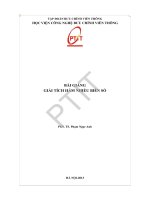
Ví dụ 1.19 Tìm một số đường mức của hàm số h(x, y) = 4x2 + y 2 . Another method for visualizing functio

map on which points of constant elevatio
curves.

TS. NGUYỄN ĐỨC HẬU

Definition The level curves of a functio
equations
f ͑x, y͒ ෇ k, where k is a con

FIGURE 6

World mean sea-level temperatures
in January in degrees Celsius

A level curve f ͑x, y͒ ෇ k is the set of a
on a given value k. In other words, it show


754

■

CHAPTER 11 PARTIAL DERIVATIVES

16

1.8. Giới hạn
củaforhàm
biếna family of ellipses with semiaxes sk͞2 and sk. Figwhich,

, describes
k Ͼ 0nhiều

ure 10(a) shows a contour map of h drawn by a computer with
level curves corre2
y 2these level curves lifted
2 +
sponding
Figure
10(b)x shows
k ෇ 0.25,
0.5, 4x
0.75,
. . .y,24.=
Giải. Phương
trìnhtođường
mức
k hay
+
=
1 (k > 0). Hình 1.11
k
k/4
up to the graph of h (an elliptic paraboloid) where they become horizontal traces.
biểu diễn một
vài đường mức với k = 0.25, 0.5, 0.75, ..., 4.
We see from Figure 10 how the graph of h is put together from the level curves.
y
z

x

x

FIGURE 10

The graph of h(x, y)=4≈+¥
is formed by lifting the level curves.

y

(a) Contour map

(b) Horizontal traces are raised level curves

Hình 1.11: Đồ thị của h(x, y) = 4x2 + y 2 .

EXAMPLE 10 Plot level curves for the Cobb-Douglas production function of
756

Example 2.

■

CHAPTER 11 PARTIAL DERIVATIVES

Ví dụ 1.20 Tìm các mặt mức của hàm số f (x, y, z) = x2 + y 2 + z 2 .

It’s very
to visualize a function f of three variables by i

SOLUTION In Figure 11 we use a computer to draw a contour plot
for difficult
the Cobbwould lie in a four-dimensional space. However, we do gain som
Douglas production function

examining
its level
surfaces,
Giải. Mặt√mức x2 + y 2 + z 2 = k với k ≥ 0. Đây là họ các
mặt cầu
đồng
tâm which
O vớiare the surfaces with equati
0.75 0.25
where k is a constant. If the point ͑x, y, z͒ moves along a level su
P͑L,
K͒
෇
1.01P
K
bán kính k (xem Hình 1.12).
f ͑x, y, z͒ remains fixed.

Level curves are labeled with the value of the production P. For instance, the level
EXAMPLE 12 Find the level surfaces of the function
curve labeled 140 shows all values of the≈+¥+z@=9
labor L and capital investment K that
z
≈+¥+z@=4
result in a production of P ෇ 140. We see that, for a fixed value of P, as L increasesf ͑x, y, z͒ ෇ x 2 ϩ y 2 ϩ z 2

K decreases, and vice versa.

SOLUTION The level surfaces are x 2 ϩ y 2 ϩ z 2 ෇ k, where k ജ 0. Th
of concentric spheres with radius sk. (See Figure 13.) Thus, as ͑x,
any sphere with center O, the value of f ͑x, y, z͒ remains fixed.

K
300
y
x

200

Hình 1.12:FIGURE
Một 13
số mặt
100

Functions of any number of variables can be considered. A funct
is a rule that assigns a number z ෇ f ͑x 1, x 2 , . . . , x n ͒ to an n-tuple
≈+¥+z@=1
real numbers. We denote by ‫ ޒ‬n the set of all such n-tuples. For exam
uses n different ingredients in making a food product, ci is the cost
220
ingredient,
mức trong
ví dụ
1.20. and x i units of the ith ingredient are used, then the total c
180
140

dients is a function of the n variables x 1, x 2 , . . . , x n :

100

C ෇ f ͑x 1, x 2 , . . . , x n ͒ ෇ c1 x 1 ϩ c2 x 2 ϩ и и и ϩ cn

3

1.8.

Giới hạn của hàm nhiều biến

FIGURE 11

100

300 L The function f is a real-valued function whose domain is a su

200

times we will use vector notation in order to write such functions m

Định nghĩa For
1.3some
Chopurposes,
hàm na biến
f (x)
f (x1 ,useful
x2 , ...,
xxn෇a) graph.

xác
trong
một
lân
we often
write
͗x
.That
. . , x nis
͘ , certainly
f ͑x͒ in place of f ͑x 1, x 2 , . . . ,
1, x 2 ,định
contour
map=
is more
than
tion
we
can
rewrite
the
function
defined
cận của điểm
(a1 , a2 10.
, ...,(Compare
an ) và LFigure
là một
số thực.
(x)in=

L ⇔ ∀ε > 0 in Equation 3 as
trueain=Example
11 with
FigureTa
3.)nói
It is lim
also f
true
estimating
x→a

function values, as in Example 6.

f ͑x͒ ෇ c ؒ x

nhỏ tuỳ ý tồnFigure
tại một
số δ > 0 sao cho khi ρ(x, a) < δ thì |f (x) − L| < ε.
12 shows some computer-generated level curves together with the corre-

where
c ෇ ͗c
c2 , . .(c)
. , ccrowd
n ͘ and c ؒ x denotes the dot product of t
sponding computer-generated graphs. Notice that the level
curves
in1,part

Định nghĩa 1.4 Giả thiết rằng hàm f (x) = f (x1 , x2 , ...,inxVInnn .)view

xácof định
với x mà sao
the one-to-one correspondence between points ͑x 1, x 2
cho ρ(x, 0) đủ lớn. Ta nói rằng lim f (x) = L nếu với ∀ε
>position
0, tồnvectors
tại sốx ෇A͗xsao
their
. . . , x n ͘ in Vn , we have three w
1, x 2 , cho
x→∞

function f defined on a subset of ‫ ޒ‬n :

khi ρ(x, 0) > A thì |ρ(x, 0) − L| < ε.

1. As a function of n real variables x 1, x 2 , . . . , x n
2. As a function of a single point variable ͑x 1, x 2 , . . . , x n ͒
3. As a function of a single vector variable x ෇ ͗x 1, x 2 , . . . , x n

TS. NGUYỄN ĐỨC HẬU



We will see that all three points of view are useful.

11.1

Exercises

●

●

●

●

●

●

●

●

●

1. In Example 1 we considered the function I ෇ f ͑T, v͒, where
I is the wind-chill index, T is the actual temperature, and v

●

●

●

●

●

●

●

●

●

●

●

●

(c) Describe in words the meaning of th
what value of T is f ͑T, 80͒ ෇ Ϫ14?


17

1.9. Sự liên tục của hàm nhiều biến số

Chú ý 1.3 Các khái niệm khác, và các định lý về phép tính giới hạn của hàm nhiều
biến cũng được định nghĩa một cách tương tự như trong lý thuyết giới hạn của hàm
số một biến.
Ví dụ 1.21 Tính các giới hạn
(a)

(b)

2x+y
lim
2
2
(x,y)→(2,3) x +y

lim

e

x sin y
y

2x+y
2
2
x→2 x +y
y→3

= lim

= lim e

=

7
3

=

lim x. siny y
x→3
e y→0

x sin y
y

x→3
y→0

(x,y)→(3,0)

lim

Ví dụ 1.22 Chứng tỏ rằng giới hạn

(x,y)→(0,0)

= e3.1 = e3

x2 +y 2
xy

không tồn tại.

Giải. Cho (x, y) → (0, 0) theo đường thẳng y = kx. Ta có:
x2 + k 2 x2
1 + k2
x2 + y 2

= lim
=
x→0
xy
kx2
k
(x,y)→(0,0)
lim

2

Giá trị này phụ thuộc vào k (chẳng hạn cho k = 1 thì 1+k
= 2, k = 2 thì
k
1+k2
k = 2.5). Vậy giới hạn của hàm đã cho không tồn tại duy nhất cho nên giới hạn
trên không tồn tại.

1.9.

Sự liên tục của hàm nhiều biến số

Định nghĩa 1.5 Ta nói hàm f (x) = f (x1 , x2 , ..., xn ) liên tục tại điểm a =
(a1 , a2 , ..., an ) ⇔ lim f (x) = f (a).
x→a

Ví dụ 1.23 (a) Hàm số ba biến
f (x1 , x2 , x3 ) =

1

1 − (x21 + x22 + x23 )

liên tục trên toàn không gian R3 trừ đi các điểm nằm trên mặt cầu x21 + x22 + x23 = 1.
Ta cũng nói rằng hàm bị gián đoạn trên mặt cầu đó.
(b) Hàm z = ln |x − y| liên tục trên toàn mặt phẳng Oxy trừ những điểm nằm
trên đường thẳng y = x. Trên đường thẳng đó hàm bị gián đoạn.

1.10.

Đạo hàm riêng

Định nghĩa 1.6 Cho hàm n biến f (x) = f (x1 , x2 , ..., xn ). Đạo hàm riêng theo biến
xi , i ∈ {1, 2, ..., n} của hàm f (x) tại điểm (x1 , x2 , ..., xn ) được xác định như sau
∂f
f (x1 , ..., xi−1 , xi + ∆xi , xi+1 , ..., xn ) − f (x1 , x2 , ..., xn )
(x1 , x2 , ..., xn ) = lim
∆xi →0
∂xi
∆xi
Một số kí hiệu khác của đạo hàm riêng fxi , fxi , Dxi f .
TS. NGUYỄN ĐỨC HẬU




18

1.10. Đạo hàm riêng

Cách tính. Khi tính đạo hàm riêng theo một biến số nào đó thì coi các biến khác

như hằng số rồi áp dụng các quy tắc tính đạo hàm của hàm số một biến số đối với
biến số đó.
Ví dụ 1.24 Tính các đạo hàm riêng của các hàm số
(a) z = x2 sin y.
z
(b) u = xy .
Giải.
(a) zx = 2x sin y, zy = x2 cos y
z
z
z
(b) ux = y z .xy −1 , uy = xy . ln x.z.y z−1 , uz = xy . ln x.y z . ln y.
Định nghĩa 1.7 Đạo hàm riêng cấp cao. Đạo hàm riêng (đhr) cấp hai là đhr
của đhr cấp 1,..., đhr cấp n là đhr của đhr cấp n − 1.
Cho hàm hai biến f (x, y). Các đạo hàm riêng cấp hai của f có thể được kí hiệu như
sau
∂
∂y
∂
∂x
∂
∂x
∂
∂y

∂f
∂x
∂f
∂y
∂f

∂x
∂f
∂y

∂2f
= fxy = fxy
∂y∂x
∂2f
=
= fyx = fyx
∂x∂y
∂2f
∂2f
=
=
= fxx = fx2 = fxx = fx2
∂x∂x
∂x2
∂2f
∂2f
=
=
= fyy = fy2 = fyy = fy2
∂y∂y
∂y 2
=

Ví dụ 1.25 Tính các đạo hàm riêng đến cấp hai của các hàm số f (x, y) = x2 y −
2xy 3 + y 4 .
Giải. fx = 2xy − 2y 3 , fy = x2 − 6xy 2 + 4y 3

2
2
fx2 = ∂∂xu2 = 2y, fy2 = ∂∂yu2 = −12xy + 12y 2 ,
fxy =

∂2u
∂x∂y

= 2x − 6y 2 , fyx =

∂2u
∂y∂x

= 2x − 6y 2 .

Chú ý 1.4 Hàm hai biến có 2k đhr cấp k, hàm ba biến có 3k đhr cấp k, ..., hàm n
biến có nk đhr cấp k.
Định lý 1.1 Clairaut. Các đhr cùng cấp, liên tục, chỉ khác nhau về thứ tự lấy đạo
hàm của cùng một hàm thì trùng nhau.
Trong ví dụ 1.25 ta có fxy = fyx .
TS. NGUYỄN ĐỨC HẬU




19

1.11. Vi phân toàn phần

1.11.

Vi phân toàn phần

Định nghĩa 1.8 Nếu tại điểm (x1 , x2 , ..., xn ) các đhr fxi , i = 1, n đều liên tục thì
hàm f (x) = f (x1 , x2 , ..., xn ) có vi phân tồn phần df (khả vi) tại điểm đó và
df (x1 , x2 , ..., xn ) = fx1 .∆x1 + fx2 .∆x2 + ... + fxn .∆xn
Ví dụ 1.26 Tìm vi phân tồn phần của hàm f (x, y) = x2 sin y tại điểm (x, y) tuỳ
ý.
Giải. Ta có fx = 2x sin y, fy = x2 cos y nên df (x, y) = 2x sin y.∆x + x2 cos y.∆y
Chú ý 1.5 Ta đã biết nếu xi là biến độc lập thì ∆xi = dxi nên cơng thức vi phân
tồn phần có thể viết lại như sau df (x1 , x2 , ..., xn ) = fx1 .dx1 + fx2 .dx2 + ... + fxn .dxn .
Định nghĩa 1.9 Vi phân toàn phần cấp cao. Vi phân toàn phần cấp hai được
xác định bởi d2 f = d(df ),..., vi phân toàn phần cấp n được xác định bởi dn f =
d(dn−1 f ).
Với hàm hai biến f (x, y) thì
d2 f = d(fx .∆x + fy ∆y)
∂ ∂f
∂f
∂ ∂f
∂f
.∆x +
.∆y .∆x +
.∆x +
.∆y .∆y
∂x ∂x
∂y
∂y ∂x
∂y
∂2f
∂2f

∂2f
2
.
(∆x)
+
2
.∆x∆y
+
. (∆y)2
=
∂x2
∂x∂y
∂y 2

=

=

∂
∂
.∆x +
.∆y
∂x
∂y

2

f

Tổng quát ta có

dn f =

∂
∂
.∆x +
.∆y
∂x
∂y

n

f

Với hàm ba biến f (x, y, z) thì
d2 f = d(fx ∆x + fy ∆y + fz ∆z)
∂ ∂f
∂f
∂f
∂ ∂f
∂f
∂f
∆x +
∆y +
∆z ∆x +
∆x +
∆y +
∆z ∆y
∂x ∂x
∂y
∂z

∂y ∂x
∂y
∂z
∂ ∂f
∂f
∂f
+
∆x +
∆y +
∆z ∆z
∂z ∂x
∂y
∂z
∂2f
∂2f
∂2f
∂2f
∂2f
2
2
2
=
(∆x)
+
(∆y)
+
(∆z)
+
2
∆x∆y

+
2
∆y∆z
∂x2
∂y 2
∂z 2
∂x∂y
∂y∂z
∂2f
+2
∆z∆x
∂z∂x
2
∂
∂
∂
=
∆x +
∆y +
∆z f
∂x
∂y
∂z
=

TS. NGUYỄN ĐỨC HẬU

20

1.12. Ứng dụng hình học

1.12.

Ứng dụng hình học

Cho mặt cong S có phương trình F (x, y, z) = 0.
Một đường thẳng được gọi là tiếp tuyến của mặt cong S tại một điểm
M (x0 , y0 , z0 ) trên mặt cong nếu nó là tiếp tuyến tại M của một đường cong nào đó
vẽ trên S đi qua M .
Tại mỗi điểm M trên mặt cong S nói chung có vơ số tiếp tuyến. Tập hợp tất cả
các tiếp tuyến với mặt cong S tại M (nếu tại M cả ba đạo hàm riêng đều tồn tại,
liên tục và không đồng thời triệt tiêu) là mặt phẳng đi qua M . Mặt phẳng đó gọi là
tiếp diện của mặt cong tại điểm ấy. Phương trình tiếp diện đó được xác định như
sau
(x − x0 )Fx (x0 , y0 , z0 ) + (y − y0 )Fy (x0 , y0 , z0 ) + (z − z0 )Fz (x0 , y0 , z0 ) = 0
Đường thẳng đi qua M và song song với véc tơ pháp tuyến của mặt phẳng tiếp diện
của S tại M gọi là pháp tuyến của S tại M . Phương trình pháp tuyến đó được xác
định như sau
x − x0
y − y0
z − z0
=
=
Fx (x0 , y0 , z0 )
Fy (x0 , y0 , z0 )
Fz (x0 , y0 , z0 )
Ví dụ 1.27 Viết phương trình pháp tuyến và tiếp diện với mặt cầu x2 +y 2 +z 2 = 14

tại điểm M (1, 2, 3).
Giải. F (x, y, z) = x2 + y 2 + z 2 − 14, Fx = 2x, Fy = 2y, Fz = 2z. Do đó Fx (M ) = 2,
Fy (M ) = 4, Fz (M ) = 6.
Phương trình pháp tuyến
x−1
y−2
z−3
=
=
2
4
6
hay là

x
y
z
= =
2
4
6

Đây là phương trình đường thẳng đi qua gốc-đường thẳng chứa một đường kính của
mặt cầu.
Phương trình tiếp diện 2(x − 1) + 4(y − 2) + 6(z − 3) = 0 hay là
x + 2y + 3z − 14 = 0

1.13.

Đạo hàm theo hướng

Cho hàm ba biến f (x, y, z). Xét M0 (x0 , y0 , z0 ) ∈ R3 . Qua M0 vẽ một đường thẳng
định hướng theo véc tơ u. Gọi M1 (x0 + ∆x, y0 + ∆y, z0 + ∆z) là một điểm nằm trên
đường thẳng định hướng.
TS. NGUYỄN ĐỨC HẬU




21

1.14. Gradient
∆x2 + ∆y 2 + ∆z 2 .

Đặt ρ = M0 M1 =

Đạo hàm theo hướng u tại điểm M0 kí hiệu là:
định như sau:

∂f
∂u (M0 )

hay Du f và được xác

∂f
f (x0 + ∆x, y0 + ∆y, z0 + ∆z) − f (x0 , y0 , z0 )
(M0 ) = lim
ρ→0
∂u
ρ

Vậy

∂f
∂u (M0 )

không những phụ thuộc vào điểm M0 mà còn phụ thuộc vào hướng

u.
Đặc biệt nếu u trùng với hướng dương của trục Ox thì
∂f
f (x0 + ρ, y0 , z0 ) − f (x0 , y0 , z0 )
∂f
(M0 ) = lim
=
(M0 )
ρ→0
∂u
ρ
∂x
Vậy

∂f
∂x (M0 )

là đạo hàm theo hướng Ox.

Tương tự ta có
hướng Oz.

∂f

∂y (M0 )

là đạo hàm theo hướng Oy và

∂f
∂z (M0 )

là đạo hàm theo

Định lý 1.2 Cho hàm f (x, y, z) khả vi tại điểm M (x, y, z) thì tại điểm đó nó có
đạo hàm theo hướng bất kì và
∂f
∂f
∂f
∂f
(M ) =
(M ) cos α +
(M ) cos β +
(M ) cos γ
∂u
∂x
∂y
∂z
trong đó cos α, cos β, cos γ là các cosine chỉ hướng của u có nghĩa là
(cos α, cos β, cos γ) //u và cos2 α + cos2 β + cos2 γ = 1.
Ví dụ 1.28 Cho hàm vơ hướng F (x, y, z) = xyz. Tính đạo hàm tại điểm M (5, 1, 2)
−−−→
theo hướng M M1 với M1 (7, −1, 3).
∂f
∂f

Giải. Ta có ∂f
∂x = yz, ∂y = xz, ∂z = xy do đó
√
−−−→
−−−→
M M1 = (2, −2, 1), M M1 = 4 + 4 + 1 = 3.

Vậy (cos α, cos β, cos γ) =

2
2 1
3, −3, 3

= 2,

∂f
∂y (M )

= 10,

∂f
∂z (M )

= 5,

nên

∂f
2
2

= 2. + 10. −
∂u
3
3

1.14.

∂f
∂x (M )

1
11
+ 5. = −
3
3

Gradient

Định nghĩa 1.10 Cho hàm số f (x, y, z). Ta gọi gradient hàm f tại M (x, y, z) là
gradf xác định như sau
gradf (M ) =

∂f
∂f
∂f
(M ),
(M ),
(M )
∂x
∂y

∂z

TS. NGUYỄN ĐỨC HẬU




22

1.14. Gradient
hay là
gradf (M ) =

∂f
∂f
∂f
(M )i +
(M )j +
(M )k
∂x
∂y
∂z

Tốn tử ∇ (del) được định nghĩa như sau
∇=

∂
∂
∂
i+

j+
k
∂x
∂y
∂z

Khi đó ta có mối liên hệ sau gradf = ∇f .
Định lý 1.3 Cho hàm số f (x, y, z) và hướng u có các cosine chỉ hướng là
cos α, cos β, cos γ. Đặt u1 = (cos α, cos β, cos γ) là véc tơ đơn vị cùng hướng với u.
Khi đó ta có
∂f
= u1 .gradf
∂u
Ví dụ 1.29 Cho hàm f (x, y, z) = x2 y 2 z 2 . Tính gradf và
−−−−→
biết rằng u là hướng của véc tơ M0 M1 với M1 (0, 1, 1).
∂f
∂x

∂f
∂y

= 2x2 yz 2 ,

tại điểm M0 (1, −1, 3)

∂f
∂z

= 2x2 y 2 z do đó gradf = 2xyz(yzi +

−−−−→
xzj + xyk) nên gradf (M0 ) = −6(−3i + 3j − k), hơn nữa M0 M1 = (−1, 2, −2) nên
∂f
= u1 .gradf ta có
u1 = − 31 , 32 , − 23 . Áp dụng cơng thức ∂u
Giải. Ta có

= 2xy 2 z 2 ,

∂f
∂u

∂f
1
(M0 ) = 18. −
∂u
3

2
2
+ (−18). + 6 −
3
3

= −22

Các tính chất
(a) grad(f1 + f2 − f3 ) = gradf1 + gradf2 − gradf3
(b) grad(c.f1 ) = cgradf1 , với c là hằng số.
(c) grad(f1 .f2 ) = f1 gradf2 + f2 gradf1

(d) gradf (u) = f (u)gradu
Chẳng hạn ta chứng minh tính chất (d). Ta có
∂
∂
∂
[f (u)] i +
[f (u)] j +
[f (u)] k
∂x
∂y
∂z
∂u
∂u
∂u
= f (u) i + f (u) j + f (u) k
∂x
∂y
∂z
= f (u)gradu

gradf (u) =

Chú ý 1.6 Hướng của véc tơ gradf trùng với hướng mà hàm f tăng nhanh nhất.
Hơn nữa tốc độ tăng nhanh nhất của f chính là độ dài của véc tơ gradf .
TS. NGUYỄN ĐỨC HẬU




23

1.15. Đạo hàm của hàm hợp

Ví dụ 1.30 Nhiệt độ khơng khí tại các điểm trong khơng gian được xác định bởi
hàm
f (x, y, z) = x2 − y + z 2
Có một con muỗi đậu tại điểm (1, 2, 1) nó nên bay theo hướng nào để được mát
nhanh nhất?
Giải. Ta có gradf = 2i − j + 2k. Bởi vì theo hướng của véc tơ gradf nhiệt độ tăng
nhanh nhất, nên con muỗi muốn được mát nhanh nhất thì nó phải bay theo hướng
806
■
CHAPTER 11 PARTIAL DERIVATIVES
−gradf = −2i + j − 2k.
z

In particular, when t ෇ t0 we have r͑t0͒ ෇ ͗x 0 , y0 , z0 ͘ , so

±F (x¸, y¸, z¸)
tangent plane
P

ٌF͑x0, y0, z0 ͒ ؒ rЈ͑t0 0

18

rê(tá)

0

S

C

y

x

FIGURE 9

Equation 18 says that the gradient vector at P, ٌF͑x0, y0, z0 ͒, is pe
tangent vector rЈ͑t0 ͒ to any curve C on S that passes through P.
ٌF͑x0, y0, z0 ͒ 0, it is therefore natural to define the tangent plan
face F͑x, y, z͒ ෇ k at P͑x 0 , y0 , z0 ͒ as the plane that passes through
vector ٌF͑x0, y0, z0 ͒. Using the standard equation of a plane (Equa
write the equation of this tangent plane as

Hình 1.13: Gradient là véc tơ pháp tuyến của mặt.
19

Fx ͑x 0 , y0 , z0 ͒͑x Ϫ x 0 ͒ ϩ Fy ͑x 0 , y0 , z0 ͒͑y Ϫ y0 ͒ ϩ Fz͑x 0 , y0 ,

Chú ý 1.7 Gradient của hàm F (x, y, z) tại điểm P0 (x0 , The
y0 , znormal
pháp
tuyến của
0 ) là line
to S at P is the line passing through P and pe
mặt mức của F qua điểm P0 .
tangent plane. The direction of the normal line is therefore given b

Ví dụ 1.31 Tìm phương trình của tiếp diện của mặt

tor ٌF͑x0, y0, z0 ͒ and so, by Equation 9.5.3, its symmetric equation
2
xy z 3 = 12 tại điểm (3, −2, 1).
x Ϫ x0
y Ϫ y0
z Ϫ z0
෇
෇
20
F
F
F
x ͑x0, y0, z0 ͒
y ͑x0, y0, z0 ͒
z͑x0, y0, z0 ͒
2 3

Giải. Mặt này là mặt mức của hàm f (x, y, z) = xy z . Véc tơ gradf tại điểm
(3, −2, 1) là véc tơ pháp tuyến của mặt tại điểm này. Véc In
tơthe
đóspecial
là: case in which the equation of a surface S is of th
2 3

3

gradf = y z i + 2xyz j +

(that is, S is the graph of a function f of two variables), we can re
2 2 as
3xy z k
F͑x, y, z͒ ෇ f ͑x, y͒ Ϫ z ෇ 0

= 4i − 12j + 36k = 4 (i − 3j + 9k)

and regard S as a level surface (with k ෇ 0) of F . Then

Do đó phương trình của tiếp diện là (x − 3) − 3(y + 2) + 9(z − 1) = 0 hay là
Fx ͑x 0 , y0 , z0 ͒ ෇ fx ͑x 0 , y0 ͒
x − 3y + 9z = 18.
Fy ͑x 0 , y0 , z0 ͒ ෇ fy ͑x 0 , y0 ͒

1.15.

Đạo hàm của hàm hợp

Fz͑x 0 , y0 , z0 ͒ ෇ Ϫ1
so Equation 19 becomes

(a) Nếu u = f (x), x = x(t, s) thì
∂u
df ∂x
=
.
∂t
dx ∂t
∂u
df ∂x

=
.
∂s
dx ∂s

fx ͑x 0 , y0 ͒͑x Ϫ x 0 ͒ ϩ fy ͑x 0 , y0 ͒͑y Ϫ y0 ͒ Ϫ ͑z Ϫ z0 ͒ ෇

(1.5)

which is equivalent to Equation 11.4.2. Thus, our new, more gene
tangent plane is consistent with the definition that was given for
Section 11.4.
(1.6)

EXAMPLE 8 Find the equations of the tangent plane and normal line

(b) Nếu u = f (x, y), x = x(t), y = y(t) thì

͑Ϫ2, 1, Ϫ3͒ to the ellipsoid

du
∂f dx ∂f dy
=
.
+
.
dt
∂x dt
∂y dt

x2

ϩ y2 ϩ
(1.7)
4

z2
෇3
9

SOLUTION The ellipsoid is the level surface (with k ෇ 3) of the funct

TS. NGUYỄN ĐỨC HẬU


F͑x, y, z͒ ෇

x2
z2
ϩ y2 ϩ
4
9


24

1.15. Đạo hàm của hàm hợp
(c) Nếu u = f (x, y), y = y(x) thì
du
∂f

∂f dy
=
+
.
dx
∂x ∂y dx

(1.8)

(d) Nếu u = f (x, y), x = x(t, s), y = y(t, s) thì
∂f ∂x ∂f ∂y
∂u
=
.
+
.
∂t
∂x ∂t
∂y ∂t
∂u
∂f ∂x ∂f ∂y
=
.
+
.
∂s
∂x ∂s
∂y ∂s

(1.9)

(1.10)

Ví dụ 1.32 Tìm các đạo hàm của các hàm hợp sau
(a) u = x3 , x = e2t sin s
(b) u = x2 + 2y, x = sin t, y = cos t
(c) u = x. sin y, y = ex

2

(d) u = x. tan y, x = e2s . cos t, y = e−2s . sin t
Giải. (a) Áp dụng công thức 1.5 và 1.6 ta có
∂u
= 3x2 .2.e2t . sin s
∂t
∂u
= 3x2 .e2t . cos s
∂s
(b) Áp dụng cơng thức 1.7 ta có
du
= 2x. cos t − 2 sin t
dt
(c) Áp dụng công thức 1.8 ta có
du
2
= sin y + x. cos y.ex .2x
dx
(d) Áp dụng cơng thức 1.9 và 1.10 ta có
∂u
x
= tan y.e2s (− sin t) +

.e−2s . cos t
∂t
cos2 y
∂u
x
= tan y.2e2s cos t +
.(−2)e−2s . sin t
∂s
cos2 y

TS. NGUYỄN ĐỨC HẬU