Changing primary energy consumption due to COVID-19: The study 20 European economies - TRƯỜNG CÁN BỘ QUẢN LÝ GIÁO DỤC THÀNH PHỐ HỒ CHÍ MINH

Bạn đang xem bản rút gọn của tài liệu. Xem và tải ngay bản đầy đủ của tài liệu tại đây (727.63 KB, 7 trang )

(1)<div class='page_container' data-page=1>

International Journal of Energy Economics and

Policy

ISSN: 2146-4553

available at http: www.econjournals.com

International Journal of Energy Economics and Policy, 2021, 11(1), 615-631.

Changing Primary Energy Consumption Due to COVID-19: The

Study 20 European Economies

Seyed Reza Mirnezami

1

*, Sajad Rajabi

2

1Assistant Professor, RISTIP, Sharif University of Technology, Tehran, Iran, 2PhD Student, Department of Economics, Imam Sadiq 
(A.S) University, Tehran, Iran. *Email:

Received: 15 July 2020 Accepted: 20 October 2020 DOI: />

ABSTRACT

With the outbreak of the coronavirus in countries around the world, governments have decided to impose restrictions and social distancing. Closures
of businesses, and hence changes in supply and demand patterns during this period, have deepened concerns among policy makers. In this article,

we investigate the change in primary energy consumption in the 20 European countries that have the highest GDP. To this end, 10 different shock

scenarios and its limitations are considered. By implementing these shocks into input-output modelling, changes in primary energy consumption are
calculated. The results show that according to the best scenario (rapid and complete economy restoration), Russia with 3.5% and Italy with 2.88%
will have the largest decrease, and according to the worst case scenario (explosive exacerbation of disease and complete quarantine), Spain with 14%
and Italy with 13% will have the largest reduction in energy consumption. In addition, considering the total changes in primary energy consumption
of these 20 countries, according to the best scenario, it will decrease by 1.81% and according to the worst-case scenario, it will decrease by 10.46%.
We discuss about possibilities that energy consumption permanently declines.

Keywords: Coronavirus, Input-output Modelling, Economy of Europe, Energy Economics

JEL Classifications: Q43, C67, D57, O13

1. INTRODUCTION

COVID-19 has become a global epidemic that has caused
devastating economic effects around the world. As the first
country to experience the virus, China is emerging from a
state of crisis, with daily satellite data on NO2 concentrations
showing a relative improvement in economic activity in the
country (Bluedorn et al., 2020). Although the state of epidemic in
European countries is still worrisome, and hence the uncertainty
is quite noticeable. According to Eurostat, the EU’s industrial

production index fell about 1.3% in the first 2 months of 2020

compared to the same period in 2019. Over the same period, the
Malta industrial production index grew by about 12.9% to the
highest growth rate and the Estonian index decreased by 6.23%
to the lowest growth rate among the EU countries. The growth of

the industrial production index during the first 2 months of 2020

has been positive for eight EU member states and negative for the
remaining 19 countries. From February 2019 to February 2020 in
the European Union, the production of capital goods decreased by
3.1%, energy by 1.7%, and intermediate goods by 0.2%.

According to the World Economic Forum, the world’s average

Effective Energy Transition index is 55.1%, the 1st time since 
2015 that it has experienced negative annual growth. According
to statistics, more than 55% of the world’s countries surveyed in
the report experienced a drop in the energy transition index. In
2020, the energy market has faced several challenges. In addition
to uncertainties about the long-term consequences of COVID-19,
a combination of disruptions, including a drop in global energy
demand, delays or downtime in energy investments and projects,
and uncertainty surrounding the employment prospects of

</div>
(2)<div class='page_container' data-page=2>

and subsequent geopolitical escalations, an unexpected volatility
in the energy market can be seen.

Considering mentioned circumstances, we intend to examine
changes in primary energy consumption in 20 major economies.
For this purpose, input-output modelling is used to measure
changes in energy consumption. Accommodating uncertainty

conditions, ten different scenarios will be considered to reflect

range of situations from complete restrictions to the complete
elimination of restrictions.

In the next section, a review of theoretical literature and studies

in this field will be done to examine the published works on this

subject and discuss the innovations of this research. In addition,

the OXCGRT index, which is used to measure the response of
governments to the prevalence of COVID-19 and the application
of restrictions in countries, is introduced to prepare the theoretical
foundations for the construction of scenarios. In the third section,
the methodology and data are presented. The fourth section
describes the results for the 20 largest economies in Europe by
GDP in 2019, followed by conclusions and policy implications.

2. FRAMEWORK

Epidemics and pandemics are one of the most stubborn, enduring,
and deadly enemies of human history, and human society has
faced many crises in the past. With COVID-19, for three billion
people (more than a third of the world’s 7.8 billion people), a
forced quarantine has been imposed due to the spread of the

coronavirus. Nonetheless, different countries have taken very
different approaches: From India, which has banned people from

leaving their homes for one and a half billion to US where the
president has said that they must return to normal life. China has
begun lifting restrictions on Wuhan and they hope to end the crisis.

2.1. Economic Impact

The failure of industries and enterprises will cause irreparable
long-term damage to the economy and the population, especially
the vulnerable population. The COVID-19 economic crisis began

as a micro-economic problem, unlike the 2008 financial crisis.

Supporting households and people in the form of existing
employee-employer relationships will help to strengthen demand and maintain
supply capacity by helping enterprises in situations where their
performance has declined, or they have been temporarily shut
down. The COVID-19 pandemic has unfavourable impact on public
health, trade, tourism, food and agriculture industries, and retail
sector, because of which governments, media, non-governmental
organizations, health professionals, communities, and individuals
are expected to have proactive approaches to address many health,
social, educational, and political issues (Evans, 2020).

COVID-19 has three main channels to affect the economy
(Boone et al., 2020). First, it impairs the supply of the economy

force, shock is created on the supply side. Consequences such as

increased layoffs and unemployment are predictable results in this

regard. Second, as a result of the outbreak of coronavirus, there is

a significant reduction in business and tourism travel, a demand for

transportation-related activities, a decrease in educational services,
and a decrease in entertainment and recreational services. This
change in demand is due to a change in consumer preferences
due to fear and thus a change in consumption patterns. The huge
result of this decline in demand is expected to be the slowdown in
money supply. Third, COVID-19 will reduce investment in goods
and services and delay investment-related decisions by creating

uncertainty about the future of the economy. In other words,
increasing global fears and uncertainty in the face of domestic and
foreign investors are delaying investment decisions.

Considering the focus of this article on energy, we need to identify

how we point to energy. There are different taxonomies for energy,

one of which is its division into primary energy and secondary energy.
Primary energy is energy that is not exposed to any conversion

process. Such as crude oil extracted from oil fields or crude natural
gas (untreated) from gas fields (Bhattacharyya, 2019). This type of

energy can be used as input feed to industrial systems and factories,
so this energy in the process is converted into more suitable forms
of energy that can be used directly by the end consumer. In another

definition, it is briefly stated that primary energy is a form of energy

that is available in nature. In contrast, secondary energy refers to
energy obtained through the process of converting primary energy.
In this study, we will study the 9 primary energies:

• Natural Gas

• Coal

• Petroleum

• Nuclear Electricity
• Hydroelectric Electricity
• Geothermal Electricity
• Wind Electricity

• Solar, Tide and Wave Electricity
• Biomass and Waste Electricity.

2.2. Government Responses

</div>
(3)<div class='page_container' data-page=3>

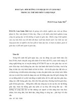
Figure 1: Government Response Tracker index

Source: FT from Blavatnik School of Government, University of Oxford

systems and manage economic consequences. The Government
Response Tracker provides a systematic international and
cross-cutting approach to understanding how the government
is progressing during the full period of the outbreak. Data is
collected from publicly available sources such as news articles,
press releases and government meetings, and recorded according

to a specific standard. The important point is that these indicators

should not be interpreted as a criterion for the appropriateness or

effectiveness of the government’s response. They do not provide

information on how policies are implemented, nor do they record

demographic or cultural characteristics that may affect the spread

of COVID-19. In addition, they are not comprehensive policy
measures. In this study, we will use this indicator to represent
economic shock intervals and to explain social constraints with
varying degrees. Figure 1 shows the index till the end of June.

3. METHODOLOGY: INPUT-OUTPUT

MODEL

In the input-output table we use in this article, the energy data is
measured by the British Thermal Unit and the non-energy data is

considered as dollar amount. To do this, first define the matrices

required for this analysis. The Z matrix is an intermediate matrix that
consists of two parts, energy carriers and non-energy materials. Total X

production and total Y demand are defined in the energy input-output

matrix. Matrix F also represents the sum of direct and indirect energy
consumption. We now calculate the A* matrix for the energy

input-output matrix using the above definitions. In this case, we will have:

( )

1
* * ˆ*

A =Z X − (1)

A matrix is a diagonal matrix in which each of the diameter

elements is the total output of one of the sectors of the economy.

For example, for a two-part economy, the Leontief coefficient

matrix will be as follows:

A

Btu Btu
Btu

* $ $

$ $

2 2

(2)
But the properties of this matrix are different from the usual
Leontief matrix. For example, the sum of each column in
matrix A* may not be <1. Direct energy consumption is the
amount of energy input that each unit receives directly from the
energy sector. The coefficients of direct energy consumption
per unit of production can be obtained using the following
equation:

F*.(X*) . *1A (3)

Total energy consumption coefficients, including direct and
indirect uses, are:

F*.(X*) .(1 I A*) 1 (4)

To investigate different types of energy consumption, we need

to distinguish between factors that are used as inputs in the
production process, such as primary energy, land and water, and
factors that are produced in this process, such as pollution. This
can be done by ecological-economic input-output analysis, in
which environmental factors can be used as inputs and outputs.
We consider a set of ecological inputs such as crude oil, gas, solar
energy, wind, biomass, water, land, etc. Each element of the matrix

M=(mkj) reflects the amount of K-type environmental input that is
used in the sector j.

</div>
(4)<div class='page_container' data-page=4>

assumed that the table has three sectors, two ecological inputs
including oil, gas and land, and two ecological outputs):

Transactions Final 
demand
Total 
Production
Ecological 
output
Consumption

Agriculture Mine Industry SO
2 HC

Production Agriculture
Mining
Industry

a11 a12 a13 f1 x1 n11 n12
a21 a22 a23 f2 x2 n21 n22

a31 a32 a33 f3 x3 n31 n32

Ecological

goods Oil and Gas Land mm1121 mm1222 mm1323

Based on this table, Leontief’s technical coefficient matrix can
be defined:

An n Zn n Xn n

(5)

Zn×n is the matrix of intermediate exchanges and Xn n

is diagonal
matrix whose diameter elements are the total production of each

sector. We then define the matrix of the coefficients of ecological
inputs. The matrix of ecological input coefficients R=[rkj] is the amount
of ecological good k used for each dollar of production in sector j.

Rk n Mk n Xn n

( ) 1 (6)

In this example, the matrix M2×3 shows the exchanges between
the two ecological goods of land and oil and gas with the sectors
of industry, agriculture and mining. The matrix of ecological

coefficients is also defined by the same method. The elements of

matrix Q=[qkj] (ecological output) represent the ecological output

k, which is produced for one dollar of the output in sector j.
Qk n Nk n Xn n

( ) 1 (7)

In this case, the matrix Nn×k is the final output of the ecological

goods that each sector of the economy produces. The matrix of

the coefficients of the total inputs and outputs of the ecological
goods is then calculated as a function of the final demand. First,
we express the matrix of coefficients of total input effects:

Qk n* Qk n (I A )n n 1 (8)

Rk n* Rk n (I A n n )1 (9)

Matrix elements Q*=[qij] indicate the amount of pollution of the
type i that is produced directly and indirectly for the supply of one

dollar of the final demand of sector j. rij* also as the element of

matrix R2 3×

* indicate how much direct and indirect ecological input

is needed to produce 1 dollar of final demand in sector j (Miller
and Blair, 2009).

Because of the social constraints imposed, it is necessary to

3.1. Partial Hypothetical Extraction Method

To study the effect of shocks, one can partially extract a sector rather

than completely extract, because there are three possible advantages

to the partial hypothetical extraction: first, it is assumed that just

α part of intermediate supply have removed to be more consistent
with what is happening in the reality of economics. Second, there
is no absolute emphasis on the intermediate matrix (quadrant I) but

instead the value-added vector and its variations are considered.
Third, there is no need to necessarily reduce the α percent of one
sector’s data, but it can be also assumed to increase the α percent
in other sectors for a variety of reasons, such as natural factors,
mining and reservoir exploration, economic policymaking (an
example of a positive shock: following the outbreak of COVID-19,
the supply of medical services has increased in many countries).
Finally, since there is no complete extraction, the intermediate
exchange matrix will not be smaller. Considering the mentioned
points, Dietzenbacher and Lahr (2013) used the partial hypothetical

extraction method to analyze the effects of capacity constraints,

for example products previously made by one sector are no
longer in demand or it is provided by suppliers from outside the
local economy, such as imports. As the output of xk decreases, the
intermediate inputs used in activity k, zik (for all i), decrease by the
same percentage. As a result, the k-column of direct needs matrix

A remain unchanged. In this case we will have:

(

)

(

)

1.2. .
ik

ik

ik ik

k k

1- a z
z

a a i n

x a x

= = = = …

− (10)

a = z
x =

- a z
- a x = a

kj kj

j

kj

j kj

1 (11)

According to (Henderson and Searle, 1981), it implies that:
L = L+ aLe b L

+ab Le
k
´
k
k
´
k
1
(12)

x - x = L - L f

(13)

f = 1- a fk

k (14)

x - x = L - L f

(15)

From the policy point of view, criteria such as employment and
value-added can be taken into consideration. The value-added
criterion is of interest to economists because it can be a good
measure of the degree of economic prosperity in society. The
well-being of individuals in society can be determined by how
much they consume. Individual consumption is a function of their
disposable income, and disposable income is also within GDP.
According to what Dietzenbacher and Lahr (2013) have calculated,
we will have to calculate total value-added changes:

VA-VA v x - x v l

i

i i i k i ik k k

</div>
(5)<div class='page_container' data-page=5>

to calculate total surplus value in all segments, the relationship

VA=×=LF can be used (Dietzenbacher and Lahr, 2013).

3.2. Data and Scenarios

We need to quantify the shock scenarios. The research conducted by
Duan et al. (2020) was used to initialize the scenarios of this study,
which is reported based on registered factual supply and demand data
in China. We use OXCGRT data set to transform China Shock to the

one for each of 20 countries based on difference between OXCGRT

indices of China and that country in 5 months of January-May. With
this strategy, we estimate shock scenarios for each country based on

real data. The present study uses the technical coefficients matrices

generated in 2015 according to Eora26 guideline. This guideline was
proposed in Lenzen et al. (2012). Also, for linking the input-output

with different types of primary energies, multiplier coefficients of

9 primary energy consumption and energy footprint of KGM and

Associates Institute were used (Table 1).

Input-Output tables of this study have been divided into 26 sectors,
described in Table 2.

Since the current situation of the countries due to COVID-19
prevalence and related limitations is in uncertainty, we will

examine 10 different scenarios in this article and model the state

of energy consumption in each case. These ten scenarios are:
• Scenario 1: Complete improvement in July and cessation of

all restrictions until the end of the year

• Scenario 2: Gradual improvement of the disease and removal
of bans and restrictions gradually to zero by the end of the
year

• Scenario 3: Gradual reduction of the epidemic by the end of
the year, but the persistence of the disease and some limitations
at a low level

• Scenario 4: Reduction of the epidemic from June and its peak
twice in the beginning of autumn (if the second wave is weaker
than March to May)

• Scenario 5: Reduction of the epidemic from June and its peak
twice in the beginning of autumn (if the second wave is like
from March to May)

• Scenario 6: Reduction of the epidemic from June and its peak
twice in the beginning of autumn (if the second wave is more
severe than March to May)

• Scenario 7: Continuation of restrictions until the end of the
year as March to May

• Scenario 8: Gradual progress of the epidemic and the
application of gradual restrictions

• Scenario 9: Epidemic progress so that it grows until October
and then full quarantine is applied

• Scenario 10: Epidemic bounds (complete quarantine from
June to the end of the year).

It should be noted that there are two important assumptions. We
assume that from 2015 to the present, the production technologies

have not changed (in other words, the technical coefficients of

the sectors are the same from 2015 to the present). In addition,
it is assumed that with respect to COVID-19 and government

decisions, the intensification of the epidemic and social constraints/
prohibition are positively correlated. The effect of temperature has

not been also considered.

4. RESULTS AND DISCUSSIONS

The average estimates of OPEC, the International Energy Agency
and the US Energy Information Administration for global oil
demand growth in 2018 were 1.3 million barrels per day and in
2019, equivalent to 700,000 barrels per day. At the beginning of
2020, it was estimated that the growth rate of demand in 2020
would reach 1.2 million barrels per day, but the prevalence and
spread of COVID-19 led to some changes in the estimates. The
OPEC and International Energy Agency indicated in April 2020
that energy demand declines sharply and unprecedentedly by the
end of 2020, dropping an average of 7.1 million barrels per day.
Since 60% of the world’s oil production is spent on transportation,

Table 1: 20 European countries studied that had the 
largest economies (GDP) in 2019

Country Abbreviation Country Abbreviation

Austria AUT Norway NOR

Belgium BEL Poland POL

Czech Republic CZE Portugal PRT

Denmark DNK Romania ROU

Finland FIN Russia RUS

France FRA Spain ESP

Germany DEU Sweden SWE

Ireland IRL Switzerland CHE

Italy ITA Turkey TUR

Netherlands NLD United Kingdom GBR

Table 2: Sectors of aggregated input-output tables

Sector Code Sector Code

Agriculture Sector 1 Construction Sector 14

Fishing Sector 2 Maintenance and Repair Sector 15

Mining and Quarrying Sector 3 Wholesale Trade Sector 16

Food and Beverages Sector 4 Retail Trade Sector 17

Textiles and Wearing Apparel Sector 5 Hotels and Restaurants Sector 18

Wood and Paper Sector 6 Transport Sector 19

Petroleum, Chemical and Non-Metallic Mineral Products Sector 7 Post and Telecommunications Sector 20

Metal Products Sector 8 Financial Intermediation and Business Activities Sector 21

Electrical and Machinery Sector 9 Public Administration Sector 22

Transport Equipment Sector 10 Education, Health and Other Services Sector 23

Other Manufacturing Sector 11 Private Households Sector 24

Recycling Sector 12 Others Sector 25

</div>
(6)<div class='page_container' data-page=6>

Table 3: Changing the consumption of different types of primary energy in Austria (10 scenarios)

Primary energies Scenario

1 (%) Scenario 2 (%) Scenario 3 (%) Scenario 4 (%) Scenario 5 (%) Scenario 6 (%) Scenario 7 (%) Scenario 8 (%) Scenario 9 (%) Scenario 10 (%)

Natural Gas −0.54 −0.83 −1.08 −1.30 −1.69 −2.62 −1.90 −4.09 −5.79 −10.57

Coal −0.15 −0.29 −0.39 −0.47 −0.61 −0.94 −0.68 −1.44 −2.03 −3.64

Petroleum −0.69 −1.03 −1.32 −1.60 −2.06 −3.19 −2.32 −4.97 −7.02 −12.78

Nuclear Electricity 0.00 0.00 0.00 0.00 0.00 0.00 0.00 0.00 0.00 0.00

Hydroelectric Electricity −0.55 −0.85 −1.10 −1.34 −1.74 −2.72 −1.95 −4.28 −6.09 −11.13

Geothermal Electricity −0.63 −0.94 −1.21 −1.46 −1.90 −2.96 −2.13 −4.64 −6.58 −12.03

Wind Electricity −0.55 −0.85 −1.10 −1.34 −1.74 −2.72 −1.95 −4.28 −6.09 −11.13

Solar, Tide and Wave

Electricity −0.80 −1.16 −1.47 −1.78 −2.30 −3.57 −2.59 −5.58 −7.89 −14.39

Biomass and Waste Electricity −0.56 −0.90 −1.17 −1.42 −1.84 −2.86 −2.07 −4.48 −6.35 −11.60

Total Primary Energy −0.57 −0.88 −1.13 −1.37 −1.77 −2.75 −1.99 −4.29 −6.07 −11.07

Table 4: Changing the consumption of different types of primary energy in Belgium (10 scenarios)

Primary Energies Scenario

Natural Gas −0.29 −0.50 −0.67 −0.76 −0.94 −2.16 −1.07 −2.64 −3.13 −4.78

Coal −0.50 −0.83 −1.10 −1.24 −1.54 −3.62 −1.76 −4.43 −5.27 −8.11

Petroleum −1.03 −1.61 −2.10 −2.37 −2.93 −6.74 −3.33 −8.21 −9.73 −14.79

Nuclear Electricity 0.00 0.00 0.00 0.00 0.00 0.00 0.00 0.00 0.00 0.00

Hydroelectric

Electricity −0.55 −0.90 −1.20 −1.35 −1.67 −3.94 −1.91 −4.83 −5.75 −8.85

Geothermal Electricity −0.55 −0.90 −1.20 −1.35 −1.67 −3.94 −1.91 −4.83 −5.75 −8.85

Wind Electricity −0.55 −0.90 −1.20 −1.35 −1.67 −3.94 −1.91 −4.83 −5.75 −8.85

Solar, Tide and Wave

Electricity −0.55 −0.87 −1.15 −1.29 −1.60 −3.74 −1.83 −4.57 −5.43 −8.34

Biomass and Waste

Electricity −0.51 −0.86 −1.15 −1.30 −1.60 −3.64 −1.81 −4.45 −5.27 −8.03

Total Primary Energy −0.63 −1.02 −1.35 −1.52 −1.88 −4.35 −2.14 −5.31 −6.30 −9.63

and because most countries have adopted quarantine and travel
restrictions, fuel demand in the transportation sector has declined
sharply. This part of decline will be mitigated after lockdown, but
the return on demand in the industrial sector will take more time
and will depend on their economic situation after the Corona crisis.
In this article, an attempt has been made to consider the restrictions
and prohibitions in the 1st months of 2020 to evaluate the situation 
of the coming months, based on 10 scenarios and for 26 sectors.
Tables 3-22 show the change in the consumption of different types

of primary energy in 20 European countries. Table 23 and Figure 2
show the aggregate change for all countries. In Figures 3-11, you
can see the state of energy consumption change in the 20 countries
under 10 scenarios. As shown in these charts, in the biomass and

waste electricity consumption, the largest decrease in consumption
according to the optimistic scenario (scenario one) is for Russia

with −4.26% and in the pessimistic scenario (scenario ten) is for
Spain with −15.49%. According to the optimistic scenario, Russia
has the highest decrease in coal consumption with −3.36% and
Spain with −14.62% in the pessimistic scenario. In the geothermal

electricity consumption, the largest decrease in consumption
according to the optimistic and pessimistic scenario is for Italy with

−2.84% and −13.94% respectively. In the hydroelectric electricity

consumption, the largest reduction in consumption according to the

optimistic and pessimistic scenario is for France with −4.72% and
−17.79% respectively. In the Natural Gas consumption, the largest

decrease in consumption according to the optimistic scenario is

for Russia with −3.31% and in the pessimistic scenario for Italy

Table 5: Changing the consumption of different types of primary energy in Czech Republic (10 scenarios)

Primary Energies Scenario

Natural Gas −0.30 −0.47 −0.62 −0.71 −0.96 −1.42 −1.08 −2.32 −3.28 −5.97

Coal −0.44 −0.71 −0.93 −1.08 −1.45 −2.14 −1.63 −3.50 −4.94 −8.99

Petroleum −0.39 −0.63 −0.82 −0.95 −1.28 −1.89 −1.44 −3.09 −4.37 −7.95

Nuclear Electricity 0.00 0.00 0.00 0.00 0.00 0.00 0.00 0.00 0.00 0.00

Hydroelectric Electricity 0.00 0.00 0.00 0.00 0.00 0.00 0.00 0.00 0.00 0.00

Geothermal Electricity 0.00 0.00 0.00 0.00 0.00 0.00 0.00 0.00 0.00 0.00

</div>
(7)<div class='page_container' data-page=7>

Table 7: Changing the consumption of different types of primary energy in Finland (10 scenarios)

Primary Energies Scenario

Natural Gas −0.20 −0.56 −0.73 −0.93 −1.20 −1.72 −1.45 −3.19 −4.60 −8.66

Coal −0.27 −0.63 −0.80 −1.02 −1.31 −1.87 −1.58 −3.45 −4.96 −9.31

Petroleum −0.56 −0.88 −1.03 −1.29 −1.64 −2.30 −1.97 −4.15 −5.92 −10.99

Nuclear Electricity −0.33 −0.76 −0.97 −1.23 −1.58 −2.27 −1.91 −4.21 −6.08 −11.42

Hydroelectric Electricity −0.33 −0.76 −0.97 −1.23 −1.58 −2.27 −1.91 −4.21 −6.08 −11.42

Geothermal Electricity 0.00 0.00 0.00 0.00 0.00 0.00 0.00 0.00 0.00 0.00

Wind Electricity −0.33 −0.76 −0.97 −1.23 −1.58 −2.27 −1.91 −4.21 −6.08 −11.42

Solar, Tide and Wave

Electricity −0.32 −0.55 −0.67 −0.84 −1.07 −1.51 −1.29 −2.77 −3.98 −7.46

Biomass and Waste

Electricity −0.15 −0.54 −0.73 −0.93 −1.20 −1.72 −1.45 −3.22 −4.65 −8.79

Total Primary Energy −0.31 −0.69 −0.87 −1.10 −1.41 −2.01 −1.70 −3.70 −5.32 −9.98

Table 6: Changing the consumption of different types of primary energy in Denmark (10 scenarios)

Primary Energies Scenario

Natural Gas −0.83 −1.17 −1.45 −1.72 −2.42 −3.53 −2.31 −4.75 −5.57 −8.36

Coal −0.87 −1.23 −1.53 −1.81 −2.57 −3.76 −2.45 −5.07 −5.96 −8.95

Petroleum −0.72 −1.03 −1.28 −1.51 −2.11 −3.04 −2.02 −4.06 −4.75 −6.99

Nuclear Electricity 0.00 0.00 0.00 0.00 0.00 0.00 0.00 0.00 0.00 0.00

Hydroelectric Electricity −0.87 −1.23 −1.53 −1.82 −2.57 −3.75 −2.45 −5.06 −5.94 −8.91

Geothermal Electricity 0.00 0.00 0.00 0.00 0.00 0.00 0.00 0.00 0.00 0.00

Wind Electricity −0.91 −1.28 −1.60 −1.90 −2.69 −3.94 −2.56 −5.31 −6.25 −9.40

Solar, Tide and Wave

Electricity 0.00 0.00 0.00 0.00 0.00 0.00 0.00 0.00 0.00 0.00

Biomass and Waste

Electricity −0.84 −1.20 −1.50 −1.77 −2.51 −3.67 −2.39 −4.95 −5.82 −8.74

Total Primary Energy −0.79 −1.12 −1.39 −1.65 −2.32 −3.37 −2.22 −4.53 −5.31 −7.91

Table 8: Changing the consumption of different types of primary energy in France (10 scenarios)

Primary Energies Scenario

Natural Gas −2.14 −2.87 −3.01 −3.71 −5.48 −6.15 −5.46 −7.44 −7.95 −8.97

Coal −2.14 −2.86 −3.00 −3.70 −5.46 −6.13 −5.44 −7.41 −7.92 −8.93

Petroleum −2.14 −2.87 −3.01 −3.72 −5.48 −6.15 −5.46 −7.45 −7.96 −8.97

Nuclear Electricity −1.98 −2.69 −2.82 −3.48 −5.15 −5.78 −5.13 −6.99 −7.48 −8.43

Hydroelectric Electricity −4.72 −5.91 −6.12 −7.56 −10.99 −12.30 −10.96 −14.83 −15.82 −17.79

Geothermal Electricity −2.14 −2.87 −3.01 −3.71 −5.48 −6.14 −5.46 −7.44 −7.95 −8.96

Wind Electricity −1.91 −2.64 −2.78 −3.43 −5.10 −5.73 −5.08 −6.95 −7.44 −8.40

Solar, Tide and Wave

Electricity −1.95 −2.63 −2.75 −3.40 −5.01 −5.63 −5.00 −6.81 −7.28 −8.20

Biomass and Waste

Electricity −2.14 −2.87 −3.01 −3.71 −5.48 −6.15 −5.46 −7.44 −7.95 −8.97

Total Primary Energy −2.15 −2.88 −3.02 −3.73 −5.50 −6.17 −5.48 −7.47 −7.99 −9.00

Table 9: Changing the consumption of different types of primary energy in Germany (10 scenarios)

Primary Energies Scenario

Natural Gas −0.34 −0.59 −0.76 −0.88 −1.18 −1.68 −1.39 −2.94 −4.03 −7.30

Coal −0.36 −0.65 −0.84 −0.98 −1.32 −1.89 −1.56 −3.33 −4.58 −8.32

Petroleum −0.80 −1.22 −1.50 −1.74 −2.33 −3.28 −2.73 −5.67 −7.72 −13.69

Nuclear Electricity −0.44 −0.76 −0.98 −1.13 −1.54 −2.20 −1.82 −3.89 −5.37 −9.80

Hydroelectric Electricity −0.44 −0.76 −0.98 −1.13 −1.54 −2.20 −1.82 −3.89 −5.37 −9.80

Geothermal Electricity −0.37 −0.61 −0.77 −0.89 −1.20 −1.72 −1.42 −3.02 −4.17 −7.61

Wind Electricity −0.44 −0.76 −0.98 −1.13 −1.54 −2.20 −1.82 −3.89 −5.37 −9.80

Solar, Tide and Wave

Electricity −0.43 −0.73 −0.94 −1.09 −1.47 −2.10 −1.74 −3.71 −5.12 −9.34

Biomass and Waste

Electricity −0.44 −0.78 −1.00 −1.16 −1.57 −2.23 −1.85 −3.93 −5.41 −9.80

</div>

Changing primary energy consumption due to COVID-19: The study 20 European economies - TRƯỜNG CÁN BỘ QUẢN LÝ GIÁO DỤC THÀNH PHỐ HỒ CHÍ MINH

<b>International Journal of Energy Economics and </b>

<b>Policy</b>

ISSN: 2146-4553

available at http: www.econjournals.com

<b>Changing Primary Energy Consumption Due to COVID-19: The </b>

<b>Study 20 European Economies</b>

<b>Seyed Reza Mirnezami</b>

<b><sub>*, Sajad Rajabi</sub></b>

<b>1. INTRODUCTION</b>

<b>2. FRAMEWORK</b>

<b>3. METHODOLOGY: INPUT-OUTPUT </b>

<b>MODEL</b>

( )

(

)

(

)

<b>4. RESULTS AND DISCUSSIONS</b>

Tài liệu liên quan

Tài liệu bạn tìm kiếm đã sẵn sàng tải về