Support Vector Machine active learning

Bạn đang xem bản rút gọn của tài liệu. Xem và tải ngay bản đầy đủ của tài liệu tại đây (302.42 KB, 22 trang )

(1)<div class='page_container' data-page=1>

Support Vector Machine Active Learning

with Applications to Text Classiﬁcation

Simon Tong

Daphne Koller

Computer Science Department
Stanford University

Stanford CA 94305-9010, USA

Editor:Leslie Pack Kaelbling

Abstract

Support vector machines have met with signiﬁcant success in numerous real-world learning
tasks. However, like most machine learning algorithms, they are generally applied using
a randomly selected training set classiﬁed in advance. In many settings, we also have the
option ofusing pool-based active learning. Instead ofusing a randomly selected training
set, the learner has access to a pool ofunlabeled instances and can request the labels for
some number of them. We introduce a new algorithm for performing active learning with
support vector machines, i.e., an algorithm for choosing which instances to request next.
We provide a theoretical motivation for the algorithm using the notion of aversion space.
We present experimental results showing that employing our active learning method can
signiﬁcantly reduce the need for labeled training instances in both the standard inductive
and transductive settings.

Keywords: Active Learning, Selective Sampling, Support Vector Machines,
Classiﬁca-tion, Relevance Feedback

1. Introduction

In many supervised learning tasks, labeling instances to create a training set is
time-consuming and costly; thus, ﬁnding ways to minimize the number oflabeled instances
is beneﬁcial. Usually, the training set is chosen to be a random sampling ofinstances.
How-ever, in many cases active learning can be employed. Here, the learner can actively choose
the training data. It is hoped that allowing the learner this extra ﬂexibility will reduce the
learner’s need for large quantities of labeled data.

Pool-based active learning for classiﬁcation was introduced by Lewis and Gale (1994).
The learner has access to a pool ofunlabeled data and can request the true class label for
a certain number ofinstances in the pool. In many domains this is a reasonable approach
since a large quantity ofunlabeled data is readily available. The main issue with active
learning is ﬁnding a way to choose good requests orqueriesfrom the pool.

Examples ofsituations in which pool-based active learning can be employed are:

</div>
(2)<div class='page_container' data-page=2>

classiﬁer that will eventually be used to classify the rest of the web. Since human
expertise is a limited resource, the company wishes to reduce the number ofpages
the employees have to label. Rather than labeling pages randomly drawn from the
web, the computer requests targeted pages that it believes will be most informative
to label.

• Email ﬁltering. The user wishes to create a personalized automatic junk email ﬁlter.
In the learning phase the automatic learner has access to the user’s past email ﬁles.
It interactively brings up past email and asks the user whether the displayed email is
junk mail or not. Based on the user’s answer it brings up another email and queries
the user. The process is repeated some number oftimes and the result is an email
ﬁlter tailored to that speciﬁc person.

• Relevance feedback. The user wishes to sort through a database or website for
items (images, articles, etc.) that are ofpersonal interest—an “I’ll know it when I
see it” type ofsearch. The computer displays an item and the user tells the learner
whether the item is interesting or not. Based on the user’s answer, the learner brings
up another item from the database. After some number of queries the learner then
returns a number ofitems in the database that it believes will be ofinterest to the
user.

The ﬁrst two examples involve induction. The goal is to create a classiﬁer that works
well on unseen future instances. The third example is an example oftransduction(Vapnik,
1998). The learner’s performance is assessed on the remaining instances in the database
rather than a totally independent test set.

We present a new algorithm that performs pool-based active learning with support
vector machines (SVMs). We provide theoretical motivations for our approach to choosing
the queries, together with experimental results showing that active learning with SVMs can
signiﬁcantly reduce the need for labeled training instances.

We shall use text classiﬁcation as a running example throughout this paper. This is
the task ofdetermining to which pre-deﬁned topic a given text document belongs. Text
classiﬁcation has an important role to play, especially with the recent explosion ofreadily
available text data. There have been many approaches to achieve this goal (Rocchio, 1971,
Dumais et al., 1998, Sebastiani, 2001). Furthermore, it is also a domain in which SVMs
have shown notable success (Joachims, 1998, Dumais et al., 1998) and it is ofinterest to
see whether active learning can oﬀer further improvement over this already highly eﬀective
method.

</div>
(3)<div class='page_container' data-page=3>

(a) (b)

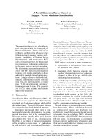
Figure 1: (a) A simple linear support vector machine. (b) A SVM (dotted line) and a

transductive SVM (solid line). Solid circles represent unlabeled instances.

2. Support Vector Machines

Support vector machines (Vapnik, 1982) have strong theoretical foundations and excellent
empirical successes. They have been applied to tasks such as handwritten digit recognition,
object recognition, and text classiﬁcation.

2.1 SVMs for Induction

We shall consider SVMs in the binary classiﬁcation setting. We are given training data

{x1. . .xn}that are vectors in some spaceX ⊆Rd. We are also given their labels{y1. . . yn}

whereyi ∈ {−1,1}. In their simplest form, SVMs are hyperplanes that separate the training
data by a maximal margin (see Fig. 1a) . All vectors lying on one side ofthe hyperplane
are labeled as −1, and all vectors lying on the other side are labeled as 1. The training
instances that lie closest to the hyperplane are calledsupport vectors. More generally, SVMs
allow one to project the original training data in space X to a higher dimensional feature
space F via a Mercer kernel operator K. In other words, we consider the set ofclassiﬁers
ofthe form:

f(x) =

n

i=1

αiK(xi,x)

. (1)

When K satisﬁes Mercer’s condition (Burges, 1998) we can write: K(u,v) = Φ(u)·Φ(v)
where Φ :X → F and “·” denotes an inner product. We can then rewritef as:

f(x) =w·Φ(x), wherew=

n

i=1

αiΦ(xi). (2)

</div>
(4)<div class='page_container' data-page=4>

implicitly project the training data from X into spaces F for which hyperplanes in F
correspond to more complex decision boundaries in the original space X.

Two commonly used kernels are the polynomial kernel given by K(u,v) = (u·v+ 1)p
which induces polynomial boundaries ofdegreepin the original spaceX1and the radial basis
function kernel K(u,v) = (e−γ(u−v)·(u−v)) which induces boundaries by placing weighted
Gaussians upon key training instances. For the majority ofthis paper we will assume that
the modulus of the training data feature vectors are constant, i.e., for all training instances

xi,Φ(xi)=λfor some ﬁxed λ. The quantityΦ(xi) is always constant for radial basis
function kernels, and so the assumption has no eﬀect for this kernel. For Φ(xi) to be

constant with the polynomial kernels we require that xi be constant. It is possible to
relax this constraint on Φ(xi) and we shall discuss this at the end ofSection 4.

2.2 SVMs for Transduction

The previous subsection worked within the framework of induction. There was a labeled
training set ofdata and the task was to create a classiﬁer that would have good performance
onunseen test data. In addition to regular induction, SVMs can also be used for
transduc-tion. Here we are ﬁrst given a set ofboth labeled and unlabeled data. The learning task is
to assign labels to the unlabeled data as accurately as possible. SVMs can perform
trans-duction by ﬁnding the hyperplane that maximizes the margin relative to both the labeled
and unlabeled data. See Figure 1b for an example. Recently,transductive SVMs (TSVMs)
have been used for text classiﬁcation (Joachims, 1999b), attaining some improvements in
precision/recall breakeven performance over regular inductive SVMs.

3. Version Space

Given a set oflabeled training data and a Mercer kernelK, there is a set ofhyperplanes that
separate the data in the induced feature space F. We call this set ofconsistent hypotheses
the version space (Mitchell, 1982). In other words, hypothesis f is in version space iffor
every training instance xi with label yi we have that f(xi) >0 if yi = 1 and f(xi) <0 if
yi =−1. More formally:

Deﬁnition 1 Our set of possible hypotheses is given as:

H=

f |f(x) = w·Φ(x)

w where w∈ W

,

where our parameter space W is simply equal to F. The version space, V is then deﬁned
as:

V ={f ∈ H | ∀i∈ {1. . . n} yif(xi)>0}.

Notice that sinceH is a set of hyperplanes, there is a bijection between unit vectors w and
hypotheses f in H. Thus we will redeﬁneV as:

V ={w∈ W | w= 1, yi(w·Φ(xi))>0, i= 1. . . n}.

</div>
(5)<div class='page_container' data-page=5>

(a) (b)

Figure 2: (a) Version space duality. The surface of the hypersphere represents unit weight
vectors. Each ofthe two hyperplanes corresponds to a labeled training instance.
Each hyperplane restricts the area on the hypersphere in which consistent
hy-potheses can lie. Here, the version space is the surface segment of the hypersphere
closest to the camera. (b) An SVM classiﬁer in a version space. The dark
em-bedded sphere is the largest radius sphere whose center lies in the version space
and whose surface does not intersect with the hyperplanes. The center of the
em-bedded sphere corresponds to the SVM, its radius is proportional to the margin
ofthe SVM inF, and the training points corresponding to the hyperplanes that
it touches are the support vectors.

Note that a version space only exists ifthe training data are linearly separable in the

feature space. Thus, we require linear separability of the training data in the feature space.
This restriction is much less harsh than it might at ﬁrst seem. First, the feature space often
has a very high dimension and so in many cases it results in the data set being linearly
separable. Second, as noted by Shawe-Taylor and Cristianini (1999), it is possible to modify
any kernel so that the data in the new induced feature space is linearly separable2.

There exists a duality between the feature spaceF and the parameter spaceW (Vapnik,
1998, Herbrich et al., 2001) which we shall take advantage ofin the next section: points in

F correspond to hyperplanes inW and vice versa.

By deﬁnition, points in W correspond to hyperplanes in F. The intuition behind the
converse is that observing a training instance xi in the feature space restricts the set of
separating hyperplanes to ones that classify xi correctly. In fact, we can show that the set

</div>
(6)<div class='page_container' data-page=6>

ofallowable points w in W is restricted to lie on one side ofa hyperplane in W. More
formally, to show that points in F correspond to hyperplanes in W, suppose we are given
a new training instance xi with label yi. Then any separating hyperplane must satisfy
yi(w·Φ(xi))> 0. Now, instead ofviewing w as the normal vector ofa hyperplane in F,

think ofΦ(xi) as being the normal vector ofa hyperplane in W. Thus yi(w·Φ(xi))> 0
deﬁnes a halfspace inW. Furthermorew·Φ(xi) = 0 deﬁnes a hyperplane in W that acts
as one ofthe boundaries to version space V. Notice that the version space is a connected
region on the surface of a hypersphere in parameter space. See Figure 2a for an example.

SVMs ﬁnd the hyperplane that maximizes the margin in the feature space F. One way
to pose this optimization task is as follows:

maximizew∈F mini{yi(w·Φ(xi))}
subject to: w= 1

yi(w·Φ(xi))>0 i= 1. . . n.

By having the conditionsw= 1 and yi(w·Φ(xi))>0 we cause the solution to lie in the
version space. Now, we can view the above problem as ﬁnding the point w in the version
space that maximizes the distance: mini{yi(w·Φ(xi))}. From the duality between feature
and parameter space, and since Φ(xi) = λ , each Φ(xi)/λ is a unit normal vector ofa
hyperplane in parameter space. Because ofthe constraints yi(w·Φ(xi)) > 0 i = 1. . . n
each ofthese hyperplanes delimit the version space. The expression yi(w·Φ(xi)) can be
regarded as:

λ× the distance between the pointwand the hyperplane with normal vector Φ(xi).
Thus, we want to ﬁnd the point w∗ in the version space that maximizes the minimum
distance to any ofthe delineating hyperplanes. That is, SVMs ﬁnd the center ofthe largest
radius hypersphere whose center can be placed in the version space and whose surface does
not intersect with the hyperplanes corresponding to the labeled instances, as in Figure 2b.
The normals ofthe hyperplanes that are touched by the maximal radius hypersphere are
the Φ(xi) for which the distanceyi(w∗·Φ(xi)) is minimal. Now, taking the original rather
than the dual view, and regardingw∗ as the unit normal vector ofthe SVM and Φ(xi) as
points in feature space, we see that the hyperplanes that are touched by the maximal radius
hypersphere correspond to the support vectors (i.e., the labeled points that are closest to
the SVM hyperplane boundary).

The radius ofthe sphere is the distance from the center ofthe sphere to one ofthe
touching hyperplanes and is given by yi(w∗ ·Φ(xi)/λ) where Φ(xi) is a support vector.
Now, viewingw∗ as a unit normal vector ofthe SVM and Φ(xi) as points in feature space,
we have that the distanceyi(w∗·Φ(xi)/λ) is:

λ× the distance between support vector Φ(xi) and the hyperplane with normal vectorw,

</div>
(7)<div class='page_container' data-page=7>

4. Active Learning

In pool-based active learning we have a pool ofunlabeled instances. It is assumed that
the instancesxare independently and identically distributed according to some underlying
distributionF(x) and the labels are distributed according to some conditional distribution
P(y|x).

Given an unlabeled pool U, an active learner has three components: (f, q, X). The
ﬁrst component is a classiﬁer,f :X → {−1,1}, trained on the current set oflabeled dataX
(and possibly unlabeled instances in U too). The second component q(X) is the querying
function that, given a current labeled set X, decides which instance in U to query next.
The active learner can return a classiﬁerf after each query (online learning) or after some
ﬁxed number ofqueries.

The main diﬀerence between an active learner and a passive learner is the querying
component q. This brings us to the issue ofhow to choose the next unlabeled instance to
query. Similar to Seung et al. (1992), we use an approach that queries points so as to attempt
to reduce the size ofthe version space as much as possible. We take a myopic approach
that greedily chooses the next query based on this criterion. We also note that myopia is a
standard approximation used in sequential decision making problems Horvitz and Rutledge
(1991), Latombe (1991), Heckerman et al. (1994). We need two more deﬁnitions before we
can proceed:

Deﬁnition 2 Area(V) is the surface area that the version space V occupies on the 
hyper-spherew= 1.

Deﬁnition 3 Given an active learner , letVi denote the version space of after iqueries
have been made. Now, given the (i+ 1)th query xi+1, deﬁne:

Vi− = Vi∩ {w∈ W | −(w·Φ(xi+1))>0},

V+

i = Vi∩ {w∈ W |+(w·Φ(xi+1))>0}.

So Vi− and Vi+ denote the resultingversion spaces when the next query xi+1 is labeled as

−1 and 1 respectively.

</div>
(8)<div class='page_container' data-page=8>

Lemma 4 Suppose we have an input space X, ﬁnite dimensional feature spaceF (induced
via a kernelK), and parameter spaceW. Suppose active learner∗ always queries instances
whose correspondinghyperplanes in parameter spaceWhalves the area of the current version
space. Letbe any other active learner. Denote the version spaces of∗ andafteriqueries
as Vi∗ and Vi respectively. Let P denote the set of all conditional distributions ofy givenx.
Then,

∀i∈N+ sup

P∈PEP

[Area(Vi∗)]≤ sup

P∈PEP[Area(Vi)],

with strict inequality whenever there exists a query j ∈ {1. . . i} by that does not halve
version space Vj−1.

Proof. The proofis straightforward. The learner,∗ always chooses to query instances

that halve the version space. Thus Area(Vi∗+1) = 12Area(Vi∗) no matter what the labeling
ofthe query points are. Let r denote the dimension offeature spaceF. Then r is also the
dimension ofthe parameter spaceW. LetSrdenote the surface area of the unit hypersphere
ofdimensionr. Then, under any conditional distributionP,Area(Vi∗) =Sr/2i.

Now, suppose does not always query an instance that halves the area ofthe version
space. Then after some number, k, ofqueries ﬁrst chooses to query a point xk+1 that
does not halve the current version spaceVk. Letyk+1∈ {−1,1} correspond to the labeling
of xk+1 that will cause the larger halfofthe version space to be chosen.

Without loss ofgenerality assume Area(Vk−)>Area(Vk+) and soyk+1 =−1. Note that
Area(Vk−) +Area(Vk+) =Sr/2k, so we have that Area(Vk−)> Sr/2k+1.

Now consider the conditional distributionP0:
P0(−1|x) =

1

2 ifx=xk+1
1 ifx=xk+1 .
Then under this distribution, ∀i > k,

EP0[Area(Vi)] =

2i−k−1Area(Vk−)>

Sr

2i.

Hence,∀i > k,

sup

P∈PEP[Area(V
∗

i)]> sup
P∈PEP

[Area(Vi)].

✷

Now, suppose w∗∈ W is the unit parameter vector corresponding to the SVM that we
would have obtained had we known the actual labels of all ofthe data in the pool. We
know that w∗ must lie in each ofthe version spacesV1 ⊃ V2 ⊃ V3. . ., whereVi denotes the

version space after i queries. Thus, by shrinking the size ofthe version space as much as
possible with each query, we are reducing as fast as possible the space in whichw∗ can lie.
Hence, the SVM that we learn from our limited number of queries will lie close tow∗.

</div>
(9)<div class='page_container' data-page=9>

(a) (b)

Figure 3: (a)SimpleMargin will queryb. (b)SimpleMargin will querya.

(a) (b)

Figure 4: (a)MaxMin Margin will queryb. The two SVMs with marginsm−andm+forb

are shown. (b)Ratio Margin will query e. The two SVMs with marginsm− and
m+ foreare shown.

This discussion provides motivation for an approach where we query instances that split
the current version space into two equal parts as much as possible. Given an unlabeled
instance x from the pool, it is not practical to explicitly compute the sizes of the new
version spaces V− and V+ (i.e., the version spaces obtained when x is labeled as −1 and
+1 respectively). We next present three ways ofapproximating this procedure.

• Simple Margin. Recall from section 3 that, given some data {x1. . .xi} and labels

{y1. . . yi}, the SVM unit vectorwi obtained from this data is the center of the largest

hypersphere that can ﬁt inside the current version space Vi. The position of wi in
the version space Vi clearly depends on the shape ofthe region Vi, however it is
often approximately in the center ofthe version space. Now, we can test each ofthe
unlabeled instances x in the pool to see how close their corresponding hyperplanes
inW come to the centrally placedwi. The closer a hyperplane in W is to the point

</div>
(10)<div class='page_container' data-page=10>

in W comes closest to the vector wi. For each unlabeled instance x, the shortest
distance between its hyperplane inWand the vectorwiis simply the distance between
the feature vector Φ(x) and the hyperplane wi in F—which is easily computed by

|wi ·Φ(x)|. This results in the natural rule: learn an SVM on the existing labeled
data and choose as the next instance to query the instance that comes closest to the
hyperplane inF.

Figure 3a presents an illustration. In the stylized picture we have ﬂattened out the

surface of the unit weight vector hypersphere that appears in Figure 2a. The white
area is version space Vi which is bounded by solid lines corresponding to labeled
instances. The ﬁve dotted lines represent unlabeled instances in the pool. The circle
represents the largest radius hypersphere that can ﬁt in the version space. Note that
the edges ofthe circle do not touch the solid lines—just as the dark sphere in 2b
does not meet the hyperplanes on the surface of the larger hypersphere (they meet
somewhere under the surface). The instance b is closest to the SVM wi and so we
will choose to queryb.

• MaxMin Margin. TheSimpleMargin method can be a rather rough approximation.
It relies on the assumption that the version space is fairly symmetric and that wi is
centrally placed. It has been demonstrated, both in theory and practice, that these
assumptions can fail signiﬁcantly (Herbrich et al., 2001). Indeed, if we are not careful
we may actually query an instance whose hyperplane does not even intersect the
version space. TheMaxMin approximation is designed to overcome these problems to
some degree. Given some data {x1. . .xi} and labels {y1. . . yi}, the SVM unit vector
wi is the center ofthe largest hypersphere that can ﬁt inside the current version
space Vi and the radius mi ofthe hypersphere is proportional3 to the size ofthe
margin of wi. We can use the radius mi as an indication ofthe size ofthe version
space (Vapnik, 1998). Suppose we have a candidate unlabeled instancexin the pool.
We can estimate the relative size ofthe resulting version spaceV−by labelingxas−1,
ﬁnding the SVM obtained from addingxto our labeled training data and looking at
the size ofits margin m−. We can perform a similar calculation forV+ by relabeling

xas class +1 and ﬁnding the resulting SVM to obtain marginm+.

Since we want an equal split ofthe version space, we wishArea(V−) andArea(V+) to
be similar. Now, consider min(Area(V−),Area(V+)). It will be small ifArea(V−) and
Area(V+) are very diﬀerent. Thus we will consider min(m−, m+) as an approximation
and we will choose to query thexfor which this quantity is largest. Hence, theMaxMin

query algorithm is as follows: for each unlabeled instancexcompute the marginsm−
andm+ofthe SVMs obtained when we labelxas−1 and +1 respectively; then choose
to query the unlabeled instance for which the quantity min(m−, m+) is greatest.
Figures 3b and 4a show an example comparing theSimpleMargin andMaxMinMargin
methods.

• Ratio Margin. This method is similar in spirit to theMaxMin Margin method. We
use m− and m+ as indications ofthe sizes ofV− and V+. However, we shall try to

</div>
(11)<div class='page_container' data-page=11>

take into account the fact that the current version space Vi may be quite elongated
and for somexin the poolbothm−andm+may be small simply because ofthe shape
ofversion space. Thus we will instead look at the relative sizes of m− and m+ and
choose to query the xfor which min(mm−+,mm+−) is largest (see Figure 4b).

The above three methods are approximations to the querying component that always
halves version space. After performing some number of queries we then return a classiﬁer
by learning a SVM with the labeled instances.

The margin can be used as an indication ofthe version space size irrespective ofwhether
the feature vectors have constant modulus. Thus the explanation for theMaxMin andRatio
methods still holds even without the constraint on the modulus ofthe training feature
vectors. The Simple method can still be used when the training feature vectors do not
have constant modulus, but the motivating explanation no longer holds since the maximal
margin hyperplane can no longer be viewed as the center ofthe largest allowable sphere.
However, for the Simple method, alternative motivations have recently been proposed by
Campbell et al. (2000) that do not require the constraint on the modulus.

For inductive learning, after performing some number of queries we then return a
classi-ﬁer by learning a SVM with the labeled instances. For transductive learning, after querying
some number ofinstances we then return a classiﬁer by learning a transductive SVM with

the labeledandunlabeled instances.

5. Experiments

For our empirical evaluation ofthe above methods we used two real-world text classiﬁcation
domains: theReuters-21578 data set and theNewsgroups data set.

5.1 Reuters Data Collection Experiments

The Reuters-21578 data set4 is a commonly used collection ofnewswire stories categorized
into hand-labeled topics. Each news story has been hand-labeled with some number oftopic
labels such as “corn”, “wheat” and “corporate acquisitions”. Note that some ofthe topics
overlap and so some articles belong to more than one category. We used the 12902 articles
from the “ModApte” split of the data5 and, to stay comparable with previous studies, we
considered the top ten most frequently occurring topics. We learned ten diﬀerent binary
classiﬁers, one to distinguish each topic. Each document was represented as a stemmed,
TFIDF-weighted word frequency vector.6 Each vector had unit modulus. A stop list of
common words was used and words occurring in fewer than three documents were also
ignored. Using this representation, the document vectors had about 10000 dimensions.

We ﬁrst compared the three querying methods in the inductive learning setting. Our
test set consisted ofthe 3299 documents present in the “ModApte” test set.

4. Obtained from www.research.att.com/˜lewis.

5. TheReuters-21578 collection comes with a set of predeﬁned training and test set splits. The commonly
used“ModApte” split ﬁlters out duplicate articles and those without a labeled topic, and then uses earlier
articles as the training set and later articles as the test set.

</div>
(12)<div class='page_container' data-page=12>

Random

Simple
MaxMin
Ratio

0 20 40 60 80 100
Labeled Training Set Size

70.0
80.0
90.0
100.0

Test Set Accuracy

Full
Ratio
MaxMin
Simple
Random
Random
Simple
MaxMin
Ratio

0 20 40 60 80 100
Labeled Training Set Size

0.0
10.0
20.0

30.0
40.0
50.0
60.0
70.0
80.0
90.0
100.0

Precision/Recall Breakeven Point

Full
Ratio
MaxMin
Simple
Random
(a) (b)

Figure 5: (a) Average test set accuracy over the ten most frequently occurring topics when
using a pool size of1000. (b) Average test set precision/recall breakeven point
over the ten most frequently occurring topics when using a pool size of 1000.

Topic Simple MaxMin Ratio Equivalent
Randomsize
Earn 86.39±1.65 87.75±1.40 90.24±2.31 34
Acq 77.04±1.17 77.08±2.00 80.42±1.50 >100
Money-fx 93.82±0.35 94.80±0.14 94.83±0.13 50
Grain 95.53±0.09 95.29±0.38 95.55±1.22 13
Crude 95.26±0.38 95.26±0.15 95.35±0.21 >100
Trade 96.31±0.28 96.64±0.10 96.60±0.15 >100

Interest 96.15±0.21 96.55±0.09 96.43±0.09 >100
Ship 97.75±0.11 97.81±0.09 97.66±0.12 >100
Wheat 98.10±0.24 98.48±0.09 98.13±0.20 >100
Corn 98.31±0.19 98.56±0.05 98.30±0.19 15

Table 1: Average test set accuracy over the top ten most frequently occurring topics (most
frequent topic ﬁrst) when trained with ten labeled documents. Boldface indicates
statistical signiﬁcance.

</div>
(13)<div class='page_container' data-page=13>

Topic Simple MaxMin Ratio Equivalent
Randomsize
Earn 86.05±0.61 89.03±0.53 88.95±0.74 12
Acq 54.14±1.31 56.43±1.40 57.25±1.61 12
Money-fx 35.62±2.34 38.83±2.78 38.27±2.44 52
Grain 50.25±2.72 58.19±2.04 60.34±1.61 51
Crude 58.22±3.15 55.52±2.42 58.41±2.39 55
Trade 50.71±2.61 48.78±2.61 50.57±1.95 85
Interest 40.61±2.42 45.95±2.61 43.71±2.07 60
Ship 53.93±2.63 52.73±2.95 53.75±2.85 >100
Wheat 64.13±2.10 66.71±1.65 66.57±1.37 >100
Corn 49.52±2.12 48.04±2.01 46.25±2.18 >100

Table 2: Average test set precision/recall breakeven point over the top ten most frequently
occurring topics (most frequent topic ﬁrst) when trained with ten labeled
docu-ments. Boldface indicates statistical signiﬁcance.

SVM with a polynomial kernel ofdegree one7 learned on the labeled training documents).
We then tested the classiﬁer on the independent test set.

The above procedure was repeated thirty times for each topic and the results were

averaged. We considered the Simple Margin, MaxMin Margin and Ratio Margin querying
methods as well as a Random Sample method. The Random Sample method simply
ran-domly chooses the next query point from the unlabeled pool. This last method reﬂects what
happens in the regular passive learning setting—the training set is a random sampling of
the data.

To measure performance we used two metrics: test set classiﬁcation error and, to
stay compatible with previous Reuters corpus results, the precision/recall breakeven point
(Joachims, 1998). Precision is the percentage ofdocuments a classiﬁer labels as “relevant”
that are really relevant. Recallis the percentage ofrelevant documents that are labeled as
“relevant” by the classiﬁer. By altering the decision threshold on the SVM we can trade
pre-cision for recall and can obtain a prepre-cision/recall curve for the test set. The prepre-cision/recall
breakeven point is a one number summary ofthis graph: it is the point at which precision
equals recall.

Figures 5a and 5b present the average test set accuracy and precision/recall breakeven
points over the ten topics as we vary the number ofqueries permitted. The horizontal line
is the performance level achieved when the SVM is trained on all 1000 labeled documents
comprising the pool. Over the Reuters corpus, the three active learning methods perform
almost identically with little notable diﬀerence to distinguish between them. Each method
also appreciably outperforms random sampling. Tables 1 and 2 show the test set accuracy
and breakeven performance of the active methods after they have asked for just eight labeled
instances (so, together with the initial two random instances, they have seen ten labeled
instances). They demonstrate that the three active methods perform similarly on this

</div>
(14)<div class='page_container' data-page=14>

0 20 40 60 80 100
Labeled Training Set Size

70.0
80.0

90.0
100.0

Test Set Accuracy FullRatio

Random Balanced
Random

Random
Simple
Ratio

0 20 40 60 80 100
Labeled Training Set Size

0.0
10.0
20.0
30.0
40.0
50.0
60.0
70.0
80.0
90.0
100.0

Precision/Recall Breakeven Point

Full

Ratio
Random Balanced
Random

(a) (b)

Figure 6: (a) Average test set accuracy over the ten most frequently occurring topics when
using a pool size of1000. (b) Average test set precision/recall breakeven point
over the ten most frequently occurring topics when using a pool size of 1000.

Reutersdata set after eight queries, with theMaxMinandRatioshowing a very slight edge in
performance. The last columns in each table are of more interest. They show approximately
how many instances would be needed ifwe were to use Random to achieve the same level
ofperformance as the Ratio active learning method. In this instance, passive learning on
average requires over six times as much data to achieve comparable levels ofperformance as
the active learning methods. The tables indicate that active learning provides more beneﬁt
with the infrequent classes, particularly when measuring performance by the precision/recall
breakeven point. This last observation has also been noted before in previous empirical
tests (McCallum and Nigam, 1998).

</div>
(15)<div class='page_container' data-page=15>

(a) (b)

Figure 7: (a) Average test set accuracy over the ten most frequently occurring topics when
using a pool sizes of500 and 1000. (b) Average breakeven point over the ten
most frequently occurring topics when using a pool sizes of 500 and 1000.

even worse than pure random guessing) and is always consistently and signiﬁcantly
out-performed by the active method. This indicates that the performance gains of the active
methods are not merely due to their ability to bias the class ofthe instances they queries.
The active methods are choosing special targeted instances and approximately halfofthese

instances happen to have positive labels.

Figures 7a and 7b show the average accuracy and breakeven point ofthe Ratio method
with two diﬀerent pool sizes. Clearly theRandomsampling method’s performance will not be
aﬀected by the pool size. However, the graphs indicate that increasing the pool ofunlabeled
data will improve both the accuracy and breakeven performance of active learning. This is
quite intuitive since a good active method should be able to take advantage ofa larger pool
ofpotential queries and ask more targeted questions.

We also investigated active learning in a transductive setting. Here we queried the
points as usual except now each method (Simple and Random) returned a transductive
SVM trained on both the labeled and remaining unlabeled data in the pool. As described
by Joachims (1998) the breakeven point for a TSVM was computed by gradually altering
the number ofunlabeled instances that we wished the TSVM to label as positive. This
invovles re-learning the TSVM multiple times and was computationally intensive. Since
our setting was transduction, the performance of each classiﬁer was measured on the pool
ofdata rather than a separate test set. This reﬂects the relevance feedback transductive
inference example presented in the introduction.

</div>
(16)<div class='page_container' data-page=16>

Inductive Passive
Transductive Passive
Inductive Active
Transductive Active
20 40 60 80 100

Labeled Training Set Size
0.0
10.0
20.0
30.0

40.0
50.0
60.0
70.0
80.0
90.0
100.0

Precision/Recall Breakeven Point

Transductive Active
Inductive Active
Transductive Passive
Inductive Passive

Figure 8: Average pool set precision/recall breakeven point over the ten most frequently
occurring topics when using a pool size of1000.

Random
Simple
MaxMin
Ratio

0 20 40 60 80 100
Labeled Training Set Size

40.0
50.0
60.0
70.0

80.0
90.0
100.0

Test Set Accuracy

Full
Ratio
MaxMin
Simple
Random
Ratio
MaxMin
Simple
Random

0 20 40 60 80 100
Labeled Training Set Size

40.0
50.0
60.0
70.0
80.0
90.0
100.0

Test Set Accuracy

Full

Ratio
MaxMin
Simple
Random
(a) (b)

Figure 9: (a) Average test set accuracy over the ﬁve comp.∗ topics when using a pool size
of500. (b) Average test set accuracy for comp.sys.ibm.pc.hardware with a 500
pool size.

the same breakeven performance as a regular SVM with aSimplemethod that has only seen
20 labeled instances.

5.2Newsgroups Experiments

</div>
(17)<div class='page_container' data-page=17>

(a) (b)

Figure 10: (a) A simple example ofquerying unlabeled clusters. (b) Macro-average test
set accuracy forcomp.os.ms-windows.miscandcomp.sys.ibm.pc.hardwarewhere
Hybriduses the Ratio method for the ﬁrst ten queries and Simplefor the rest.

We placed halfofthe 5000 documents aside to use as an independent test set, and
repeatedly, randomly chose a pool of500 documents from the remaining instances. We
performed twenty runs for each of the ﬁve topics and averaged the results. We used test
set accuracy to measure performance. Figure 9a contains the learning curve (averaged
over all ofthe results for the ﬁve comp.∗ topics) for the three active learning methods
and Random sampling. Again, the horizontal line indicates the performance of an SVM
that has been trained on the entire pool. There is no appreciable diﬀerence between the
MaxMin and Ratio methods but, in two ofthe ﬁve newsgroups (comp.sys.ibm.pc.hardware
and comp.os.ms-windows.misc) the Simple active learning method performs notably worse

than the MaxMin and Ratio methods. Figure 9b shows the average learning curve for the
comp.sys.ibm.pc.hardware topic. In around ten to ﬁfteen per cent of the runs for both of
the two newsgroups the Simple method was misled and performed extremely poorly (for
instance, achieving only 25% accuracy even with ﬁfty training instances, which is worse
than just randomly guessing a label!). This indicates that theSimplequerying method may
be more unstable than the other two methods.

One reason for this could be that the Simple method tends not to explore the feature
space as aggressively as the other active methods, and can end up ignoring entire clusters
ofunlabeled instances. In Figure 10a, the Simple method takes several queries before it
even considers an instance in the unlabeled cluster while both theMaxMinand Ratioquery
a point in the unlabeled cluster immediately.

</div>
(18)<div class='page_container' data-page=18>

Query Simple MaxMin Ratio Hybrid
1 0.008 3.7 3.7 3.7
5 0.018 4.1 5.2 5.2
10 0.025 12.5 8.5 8.5
20 0.045 13.6 19.9 0.045
30 0.068 22.5 23.9 0.073
50 0.110 23.2 23.3 0.115
100 0.188 42.8 43.2 0.2

Table 3: Typical run times in seconds for the Active methods on the Newsgroupsdataset

over 20 seconds to generate the 50th query on a Sun Ultra 60 450Mhz workstation with a
pool of500 documents). However, when the quantity oflabeled data is small, even with
a large pool size, MaxMin and Ratio are fairly fast (taking a few seconds per query) since
now training each SVM is fairly cheap. Interestingly, it is in the ﬁrst ten queries that the
Simpleseems to suﬀer the most through its lack ofaggressive exploration. This motivates
a Hybrid method. We can use MaxMin or Ratio for the ﬁrst few queries and then use the

Simple method for the rest. Experiments with the Hybrid method show that it maintains
the stability ofthe MaxMin and Ratio methods while allowing the scalability oftheSimple
method. Figure 10b compares the Hybrid method with the Ratio and Simple methods on
the two newsgroups for which the Simplemethod performed poorly. The test set accuracy
ofthe Hybrid method is virtually identical to that ofthe Ratio method while the Hybrid
method’s run time was about the same as the Simplemethod, as indicated by Table 3.
6. Related Work

There have been several studies ofactive learning for classiﬁcation. The Query by
Com-mittee algorithm (Seung et al., 1992, Freund et al., 1997) uses a prior distribution over
hypotheses. This general algorithm has been applied in domains and with classiﬁers for
which specifying and sampling from a prior distribution is natural. They have been used
with probabilistic models (Dagan and Engelson, 1995) and speciﬁcally with the Naive Bayes
model for text classiﬁcation in a Bayesian learning setting (McCallum and Nigam, 1998).
The Naive Bayes classiﬁer provides an interpretable model and principled ways to
incorpo-rate prior knowledge and data with missing values. However, it typically does not perform
as well as discriminative methods such as SVMs, particularly in the text classiﬁcation
do-main (Joachims, 1998, Dumais et al., 1998).

We re-created McCallum and Nigam’s (1998) experimental setup on the Reuters-21578
corpus and compared the reported results from their algorithm (which we shall call the
MN-algorithm hereafter) with ours. In line with their experimental setup, queries were asked
ﬁve at a time, and this was achieved by picking the ﬁve instances closest to the current
hyperplane. Figure 11a compares McCallum and Nigam’s reported results with ours. The
graph indicates that the Active SVM performance is signiﬁcantly better than that of the
MN-algorithm.

</div>
(19)<div class='page_container' data-page=19>

the-0 50 100 150 200
Labeled Training Set Size

20
40
60
80
100

Precision/Recall Breakeven point SVM Simple Active

MN−Algorithm

150 300 450 600 750 900
Labeled Training Set Size

60
70
80
90
100

Test Set Accuracy

SVM Simple Active
SVM Passive

LT−Algorithm Winnow Active
LT−Algorthm Winnow Passive

(a) (b)

Figure 11: (a) Average breakeven point performance over the Corn, Trade and Acq

Reuters-21578 categories. (b) Average test set accuracy over the top tenReuters-21578
categories.

oretical justiﬁcations ofthe Query by Committee algorithm, they successfully used their
committee based active learning method with Winnow classiﬁers in the text categorization
domain. Figure 11b was produced by emulating their experimental setup on the
Reuters-21578 data set and it compares their reported results with ours. Their algorithm does
not require a positive and negative instance to seed their classiﬁer. Rather than seeding
our Active SVM with a positive and negative instance (which would give the Active SVM
an unfair advantage) the Active SVM randomly sampled 150 documents for its ﬁrst 150
queries. This process virtually guaranteed that the training set contained at least one
posi-tive instance. The Acposi-tive SVM then proceeded to query instances acposi-tively using theSimple
method. Despite the very naive initialization policy for the Active SVM, the graph shows
that the Active SVM accuracy is signiﬁcantly better than that oftheLT-algorithm.

Lewis and Gale (1994) introduced uncertainty sampling and applied it to a text domain
using logistic regression and, in a companion paper, using decision trees (Lewis and Catlett,
1994). TheSimplequerying method for SVM active learning is essentially the same as their
uncertainty sampling method (choose the instance that our current classiﬁer is most
uncer-tain about), however they provided substantially less justiﬁcation as to why the algorithm
should be eﬀective. They also noted that the performance of the uncertainty sampling
method can be variable, performing quite poorly on occasions.

</div>
(20)<div class='page_container' data-page=20>

7. Conclusions and Future Work

We have introduced a new algorithm for performing active learning with SVMs. By taking
advantage ofthe duality between parameter space and feature space, we arrived at three
algorithms that attempt to reduce version space as much as possible at each query. We
have shown empirically that these techniques can provide considerable gains in both the
inductive and transductive settings—in some cases shrinking the need for labeled instances

by over an order ofmagnitude, and in almost all cases reaching the performance achievable
on the entire pool having seen only a fraction of the data. Furthermore, larger pools of
unlabeled data improve the quality ofthe resulting classiﬁer.

Ofthe three main methods presented, theSimplemethod is computationally the fastest.
However, the Simple method seems to be a rougher and more unstable approximation, as
we witnessed when it performed poorly on two of the ﬁve Newsgroup topics. If asking each
query is expensive relative to computing time then using either theMaxMinorRatiomay be
preferable. However, ifthe cost ofasking each query is relatively cheap and more emphasis
is placed upon fast feedback then the Simplemethod may be more suitable. In either case,
we have shown that the use of these methods for learning can substantially outperform
standard passive learning. Furthermore, experiments with theHybridmethod indicate that
it is possible to combine the beneﬁts oftheRatio and Simplemethods.

The work presented here leads us to many directions ofinterest. Several studies have
noted that gains in computational speed can be obtained at the expense ofgeneralization
performance by querying multiple instances at a time (Lewis and Gale, 1994, McCallum
and Nigam, 1998). Viewing SVMs in terms ofthe version space gives an insight as to where
the approximations are being made, and this may provide a guide as to which multiple
instances are better to query. For instance, it is suboptimal to query two instances whose
version space hyperplanes are fairly parallel to each other. So, with the Simple method,
instead ofblindly choosing to query the two instances that are the closest to the current
SVM, it may be better to query two instances that are close to the current SVM and whose
hyperplanes in the version space are fairly perpendicular. Similar tradeoﬀs can be made for
theRatio and MaxMin methods.

Bayes Point Machines (Herbrich et al., 2001) approximately ﬁnd the center ofmass of
the version space. Using the Simplemethod with this point rather than the SVM point in
the version space may produce an improvement in performance and stability. The use of
Monte Carlo methods to estimate version space areas may also give improvements.

One way ofviewing the strategy ofalways choosing to halve the version space is that we
have essentially placed a uniform distribution over the current space of consistent hypotheses
and we wish to reduce the expected size ofthe version space as fast as possible. Rather
than maintaining a uniform distribution over consistent hypotheses, it is plausible that
the addition ofprior knowledge over our hypotheses space may allow us to modify our
query algorithm and provided us with an even better strategy. Furthermore, the
PAC-Bayesian framework introduced by McAllester (1999) considers the eﬀect of prior knowledge
on generalization bounds and this approach may lead to theoretical guarantees for the
modiﬁed querying algorithms.

</div>
(21)<div class='page_container' data-page=21>

labeling. However, the temporarily modiﬁed data sets will only diﬀer by one instance from
the original labeled data set and so one can envisage learning an SVM on the original data
set and then computing the “incremental” updates to obtain the new SVMs (Cauwenberghs
and Poggio, 2001) for each ofthe possible labelings ofeach ofthe unlabeled instances. Thus,
one would hopefully obtain a much more eﬃcient implementation of theRatioand MaxMin
methods and hence allow these active learning algorithms to scale up to larger problems.

Acknowledgments

This work was supported by DARPA’sInformation Assurance program under subcontract
to SRI International, and by ARO grant DAAH04-96-1-0341 under the MURI program
“Integrated Approach to Intelligent Systems”.

References

C. J.C. Burges. A tutorial on support vector machines for pattern recognition. Data Mining
and Knowledge Discovery, 2:121–167, 1998.

C. Campbell, N. Cristianini, and A. Smola. Query learning with large margin classiﬁers. In

Proceedings of the Seventeenth International Conference on Machine Learning, 2000.
G Cauwenberghs and T. Poggio. Incremental and decremental support vector machine

learning. In Advances in Neural Information ProcessingSystems, volume 13, 2001.
C. Cortes and V. Vapnik. Support vector networks. Machine Learning, 20:1–25, 1995.
I. Dagan and S. Engelson. Committee-based sampling for training probabilistic classiﬁers.

InProceedings of the Twelfth International Conference on Machine Learning, pages 150–
157. Morgan Kaufmann, 1995.

S.T. Dumais, J. Platt, D. Heckerman, and M. Sahami. Inductive learning algorithms and
representations for text categorization. In Proceedings of the Seventh International 
Con-ference on Information and Knowledge Management. ACM Press, 1998.

Y. Freund, H. Seung, E. Shamir, and N. Tishby. Selective sampling using the query by
committee algorithm. Machine Learning, 28:133–168, 1997.

D. Heckerman, J. Breese, and K. Rommelse. Troubleshooting Under Uncertainty. Technical
Report MSR-TR-94-07, Microsoft Research, 1994.

R. Herbrich, T. Graepel, and C. Campbell. Bayes point machines. Journal of Machine
LearningResearch, pages 245–279, 2001.

E. Horvitz and G. Rutledge. Time dependent utility and action under uncertainty. In
Proceedings of the Seventh Conference on Uncertainty in Artiﬁcial Intelligence. Morgan
Kaufmann, 1991.

</div>
(22)<div class='page_container' data-page=22>

T. Joachims. Making large-scale svm learning practical. In B. Schăolkopf, C. Burges, and
A. Smola, editors, Advances in Kernel Methods - Support Vector Learning. MIT Press,
1999a.

T. Joachims. Transductive inference for text classiﬁcation using support vector machines.
In Proceedings of the Sixteenth International Conference on Machine Learning, pages
200–209. Morgan Kaufmann, 1999b.

K. Lang. Newsweeder: Learning to ﬁlter netnews. InInternational Conference on Machine
Learning, pages 331–339, 1995.

Jean-Claude Latombe. Robot Motion Planning. Kluwer Academic Publishers, 1991.
D. Lewis and J. Catlett. Heterogeneous uncertainty sampling for supervised learning. In

Proceedings of the Eleventh International Conference on Machine Learning, pages 148–
156. Morgan Kaufmann, 1994.

D. Lewis and W. Gale. A sequential algorithm for training text classiﬁers. In 
Proceed-ings of the Seventeenth Annual International ACM-SIGIR Conference on Research and
Development in Information Retrieval, pages 3–12. Springer-Verlag, 1994.

D. McAllester. PAC-Bayesian model averaging. In Proceedings of the Twelfth Annual
Conference on Computational LearningTheory, 1999.

A. McCallum. Bow: A toolkit for statistical language modeling, text retrieval, classiﬁcation
and clustering. www.cs.cmu.edu/˜mccallum/bow, 1996.

A. McCallum and K. Nigam. Employing EM in pool-based active learning for text
classi-ﬁcation. In Proceedings of the Fifteenth International Conference on Machine Learning.
Morgan Kaufmann, 1998.

T. Mitchell. Generalization as search. Artiﬁcial Intelligence, 28:203–226, 1982.

J. Rocchio. Relevance feedback in information retrieval. In G. Salton, editor,The SMART
retrieval system: Experiments in automatic document processing. Prentice-Hall, 1971.
G. Schohn and D. Cohn. Less is more: Active learning with support vector machines. In

Proceedings of the Seventeenth International Conference on Machine Learning, 2000.
Fabrizio Sebastiani. Machine learning in automated text categorisation. Technical Report

IEI-B4-31-1999, Istituto di Elaborazione dell’Informazione, 2001.

H.S. Seung, M. Opper, and H. Sompolinsky. Query by committee. In Proceedings of
Computational LearningTheory, pages 287–294, 1992.

J. Shawe-Taylor and N. Cristianini. Further results on the margin distribution. In 
Pro-ceedings of the Twelfth Annual Conference on Computational Learning Theory, pages
278–285, 1999.

</div>

Support Vector Machine active learning

<b>Support Vector Machine Active Learning</b>

<b>with Applications to Text Classiﬁcation</b>

Tài liệu liên quan

Tài liệu bạn tìm kiếm đã sẵn sàng tải về