Tài liệu Multimedia Data Mining 3 pdf
Bạn đang xem bản rút gọn của tài liệu. Xem và tải ngay bản đầy đủ của tài liệu tại đây (989.42 KB, 71 trang )
Chapter 3
Statistical Mining Theory and
Techniques
3.1 Introduction
Multimedia data mining is an interdisciplinary research field in which generic
data mining theory and techniques are applied to the multimedia data to fa-
cilitate multimedia-specific knowledge discovery tasks. In this chapter, com-
monly used and recently developed generic statistical learning theory, con-
cepts, and techniques in recent multimedia data mining literature are intro-
duced and their pros and cons are discussed. The principles and uniqueness
of the applications of these statistical data learning and mining techniques to
the multimedia domain are also provided in this chapter.
Data mining is defined as discovering hidden information in a data set.
Like data mining in general, multimedia data mining involves many different
algorithms to accomplish different tasks. All of these algorithms attempt to fit
a model to the data. The algorithms examine the data and determine a model
that is closest to the characteristics of the data being examined. Typical data
mining algorithms can be characterized as consisting of three components:
• Model: The purpose of the algorithm is to fit a model to the data.
• Preference: Some criteria must be used to select one model over another.
• Search: All the algorithms require searching the data.
The model in data mining can be either predictive or descriptive in nature. A
predictive model makes a prediction about values of data using known results
found from different data sources. A descriptive model identifies patterns or
relationships in data. Unlike the predictive model, a descriptive model serves
as a way to explore the properties of the data examined, not to predict new
properties.
There are many different statistical methods used to accommodate different
multimedia data mining tasks. These methods not only require specific types
of data structures, but also imply certain types of algorithmic approaches.
The statistical learning theory and techniques introduced in this chapter are
the ones that are commonly used in practice and/or recently developed in
71
© 2009 by Taylor & Francis Group, LLC
72 Multimedia Data Mining
the literature to perform specific multimedia data mining tasks as exemplified
in the subsequent chapters of the book. Specifically, in the multimedia data
mining context, the classification and regression tasks are especially perva-
sive, and the data-driven statistical machine learning theory and techniques
are particularly important. Two major paradigms of statistical learning mod-
els that are extensively used in the recent multimedia data mining litera-
ture are studied and introduced in this chapter: the generative models and
the discriminative models. In the generative models, we mainly focus on
the Bayesian learning, ranging from the classic Naive Bayes Learning, to the
Belief Networks, to the most recently developed graphical models including
Latent Dirichlet Allocation, Probabilistic Latent Semantic Analysis, and Hi-
erarchical Dirichlet Process. In the discriminative models, we focus on the
Support Vector Machines, as well as its recent development in the context of
multimedia data mining on maximum margin learning with structured out-
put space, and the Boosting theory for combining a series of weak classifiers
into a stronger one. Considering the typical special application requirements
in multimedia data mining where it is common that we encounter ambigui-
ties and/or scarce training samples, we also introduce two recently developed
learning paradigms: multiple instance learning and semi-supervised learning,
with their applications in multimedia data mining. The former addresses the
training scenario when ambiguities are present, while the latter addresses the
training scenario when there are only a few training samples available. Both
these scenarios are very common in multimedia data mining and, therefore,
it is important to include these two learning paradigms into this chapter.
The remainder of this chapter is organized as follows. Section 3.2 intro-
duces Bayesian learning. A well-studied statistical analysis technique, Prob-
abilistic Latent Semantic Analysis, is introduced in Section 3.3. Section 3.4
introduces another related statistical analysis technique, Latent Dirichlet Al-
location (LDA), and Section 3.5 introduces the most recent extension of LDA
to a hierarchical learning model called Hierarchical Dirichlet Process (HDP).
Section 3.6 briefly reviews the recent literature in multimedia data mining
using these generative latent topic discovery techniques. Afterwards, an im-
portant, and probably the most important, discriminative learning model,
Support Vector Machines, is introduced in Section 3.7. Section 3.8 introduces
the recently developed maximum margin learning theory in the structured
output space with its application in multimedia data mining. Section 3.9
introduces the boosting theory to combine multiple weak learners to build
a strong learner. Section 3.10 introduces the recently developed multiple
instance learning theory and its applications in multimedia data mining. Sec-
tion 3.11 introduces another recently developed learning theory with extensive
multimedia data mining applications called semi-supervised learning. Finally,
this chapter is summarized in Section 3.12.
© 2009 by Taylor & Francis Group, LLC
Statistical Mining Theory and Techniques 73
3.2 Bayesian Learning
Bayesian reasoning provides a probabilistic approach to inference. It is
based on the assumption that the quantities of interest are governed by prob-
ability distribution and that an optimal decision can be made by reasoning
about these probabilities together with observed data. A basic familiarity
with Bayesian methods is important to understand and characterize the oper-
ation of many algorithms in machine learning. Features of Bayesian learning
methods include:
• Each observed training example can incrementally decrease or increase
the estimated probability that a hypothesis is correct. This provides
a more flexible approach to learning than algorithms that completely
eliminate a hypothesis if it is found to be inconsistent with any single
example.
• Prior knowledge can be combined with the observed data to determine
the final probability of a hypothesis. In Bayesian learning, prior knowl-
edge is provided by asserting (1) a prior probability for each candidate
hypothesis, and (2) a probability distribution over the observed data for
each possible hypothesis.
• Bayesian methods can accommodate hypotheses that make probabilistic
predictions (e.g., the hypothesis such as “this email has a 95% proba-
bility of being spam”).
• New instances can be classified by combining the predictions of multiple
hypotheses, weighted by their probabilities.
• Even in cases where Bayesian methods prove computationally intractable,
they can provide a standard of optimal decision making against which
other practical methods can be measured.
3.2.1 Bayes Theorem
In multimedia data mining we are often interested in determining the best
hypothesis from a space H, given the observed training data D. One way
to specify what we mean by the best hypothesis is to say that we demand
the most probable hypothesis, given the data D plus any initial knowledge
about the prior probabilities of the various hypotheses in H. Bayes theorem
provides a direct method for calculating such probabilities. More precisely,
Bayes theorem provides a way to calculate the probability of a hypothesis
based on its prior probability, the probabilities of observing various data given
the hypothesis, and the observed data themselves.
© 2009 by Taylor & Francis Group, LLC
74 Multimedia Data Mining
First, let us introduce the notations. We shall write P (h) to denote the
initial probability that hypothesis h holds true, before we have observed the
training data. P (h) is often called the prior probability of h and may reflect
any background knowledge we have about the chance that h is a correct
hypothesis. If we have no such prior knowledge, then we might simply assign
the same prior probability to each candidate hypothesis. Similarly, we will
write P (D) to denote the prior probability that training data set D is observed
(i.e., the probability of D given no knowledge about which the hypothesis
holds true). Next we write P (D|h) to denote the probability of observing
data D given a world in which hypothesis h holds true. More generally, we
write P (x|y) to denote the probability of x given y. In machine learning
problems we are interested in the probability P (h|D) that h holds true given
the observed training data D. P (h|D) is called the posterior probability of
h, because it reflects our confidence that h holds true after we have seen
the training data D. Note that the posterior probability P (h|D) reflects the
influence of the training data D, in contrast to the prior probability P (h),
which is independent of D.
Bayes theorem is the cornerstone of Bayesian learning methods because it
provides a way to compute the posterior probability P (h|D) from the prior
probability P (h), together with P (D) and P (D|h). Bayes Theorem states:
THEOREM 3.1
P (h|D) =
P (D|h)P (h)
P (D)
(3.1)
As one might intuitively expect, P (h|D) increases with P (h) and with
P (D|h), according to Bayes theorem. It is also reasonable to see that P (h|D)
decreases as P (D) increases, because the more probably D is observed inde-
pendent of h, the less evidence D provides in support of h.
In many classification scenarios, a learner considers a set of candidate hy-
potheses H and is interested in finding the most probable hypothesis h ∈ H
given the observed data D (or at least one of the maximally probable hypothe-
ses if there are several). Any such maximally probable hypothesis is called a
maximum a posteriori (MAP) hypothesis. We can determine the MAP hy-
potheses by using Bayes theorem to compute the posterior probability of each
candidate hypothesis. More precisely, we say that h
MAP
is a MAP hypothesis
provided
h
MAP
= arg max
h∈H
P (h|D)
= arg max
h∈H
P (D|h)P (h)
P (D)
= arg max
h∈H
P (D|h)P (h) (3.2)
© 2009 by Taylor & Francis Group, LLC
Statistical Mining Theory and Techniques 75
Notice that in the final step above we have dropped the term P (D) because
it is a constant independent of h.
Sometimes, we assume that every hypothesis in H is equally probable a
priori (P (h
i
) = P (h
j
) for all h
i
and h
j
in H). In this case we can further
simplify Equation 3.2 and need only consider the term P (D|h) to find the
most probable hypothesis. P (D|h) is often called the likelihood of the data
D given h, and any hypothesis that maximizes P (D|h) is called a maximum
likelihood (ML) hypothesis, h
ML
.
h
ML
≡ arg max
h∈H
P (D|h) (3.3)
3.2.2 Bayes Optimal Classifier
The previous section introduces Bayes theorem by considering the question
“What is the most probable hypothesis given the training data?” In fact,
the question that is often of most significance is the closely related question
“What is the most probable classification of the new instance given the train-
ing data?” Although it may seem that this second question can be answered
by simply applying the MAP hypothesis to the new instance, in fact, it is
possible to even do things better.
To develop an intuition, consider a hypothesis space containing three hy-
potheses, h
1
, h
2
, and h
3
. Suppose that the posterior probabilities of these
hypotheses given the training data are 0.4, 0.3, and 0.3, respectively. Thus,
h
1
is the MAP hypothesis. Suppose a new instance x is encountered, which is
classified positive by h
1
but negative by h
2
and h
3
. Taking all hypotheses into
account, the probability that x is positive is 0.4 (the probability associated
with h
1
), and the probability that it is negative is therefore 0.6. The most
probable classification (negative) in this case is different from the classification
generated by the MAP hypothesis.
In general, the most probable classification of a new instance is obtained
by combining the predictions of all hypotheses, weighted by their posterior
probabilities. If the possible classification of the new example can take on
any value v
j
from a set V , then the probability P (v
j
|D) that the correct
classification for the new instance is v
j
is just
P (v
j
|D) =
h
i
∈H
P (v
j
|h
i
)P (h
i
|D)
The optimal classification of the new instance is the value v
j
, for which
P (v
j
|D) is maximum. Consequently, we have the Bayes optimal classification:
arg max
v
j
∈V
h
i
∈H
P (v
j
|h
i
)P (h
i
|D) (3.4)
Any system that classifies new instances according to Equation 3.4 is called
a Bayes optimal classifier, or Bayes optimal learner. No other classification
© 2009 by Taylor & Francis Group, LLC
76 Multimedia Data Mining
method using the same hypothesis space and the same prior knowledge can
outperform this method on average. This method maximizes the probability
that the new instance is classified correctly, given the available data, hypoth-
esis space, and prior probabilities over the hypotheses.
Note that one interesting property of the Bayes optimal classifier is that
the predictions it makes can correspond to a hypothesis not contained in H.
Imagine using Equation 3.4 to classify every instance in X. The labeling of
instances defined in this way need not correspond to the instance labeling of
any single hypothesis h from H. One way to view this situation is to think
of the Bayes optimal classifier as effectively considering a hypothesis space
H
′
different from the space of hypotheses H to which Bayes theorem is being
applied. In particular, H
′
effectively includes hypotheses that perform com-
parisons between linear combinations of predictions from multiple hypotheses
in H.
3.2.3 Gibbs Algorithm
Although the Bayes optimal classifier obtains the best performance that can
be achieved from the given training data, it may also be quite costly to apply.
The expense is due to the fact that it computes the posterior probability for
every hypothesis in H and then combines the predictions of each hypothesis
to classify each new instance.
An alternative, less optimal method is the Gibbs algorithm [161], defined
as follows:
1. Choose a hypothesis h from H at random, according to the posterior
probability distribution over H.
2. Use h to predict the classification of the next instance x.
Given a new instance to classify, the Gibbs algorithm simply applies a
hypothesis drawn at random according to the current posterior probability
distribution. Surprisingly, it can be shown that under certain conditions the
expected misclassification error for the Gibbs algorithm is at most twice the
expected error of the Bayes optimal classifier. More precisely, the expected
value is taken over target concepts drawn at random according to the prior
probability distribution assumed by the learner. Under this condition, the ex-
pected value of the error of the Gibbs algorithm is at worst twice the expected
value of the error of the Bayes optimal classifier.
3.2.4 Naive Bayes Classifier
One highly practical Bayesian learning method is the naive Bayes learner,
often called the naive Bayes classifier. In certain domains its performance
has been shown to be comparable to those of neural network and decision
tree learning.
© 2009 by Taylor & Francis Group, LLC
Statistical Mining Theory and Techniques 77
The naive Bayes classifier applies to learning tasks where each instance x is
described by a conjunction of attribute values and where the target function
f(x) can take on any value from a finite set V . A set of training examples of
the target function is provided, and a new instance is presented, described by
the tuple of attribute values (a
1
, a
2
, ..., a
n
). The learner is asked to predict
the target value, or classification, for this new instance.
The Bayesian approach to classifying the new instance is to assign the most
probable target value, v
MAP
, given the attribute values (a
1
, a
2
, ..., a
n
) that
describe the instance.
v
MAP
= arg max
v
j
∈V
P (v
j
|a
1
, a
2
, ..., a
n
)
We can use Bayes theorem to rewrite this expression as
v
MAP
= arg max
v
j
∈V
P (a
1
, a
2
, ..., a
n
|v
j
)P (v
j
)
P (a
1
, a
2
, ..., a
n
)
= arg max
v
j
∈V
P (a
1
, a
2
, ..., a
n
|v
j
)P (v
j
) (3.5)
Now we can attempt to estimate the two terms in Equation 3.5 based on the
training data. It is easy to estimate each of the P (v
j
) simply by counting the
frequency in which each target value v
j
occurs in the training data. However,
estimating the different P (a
1
, a
2
, ..., a
n
|v
j
) terms in this fashion is not feasible
unless we have a very large set of training data. The problem is that the
number of these terms is equal to the number of possible instances times the
number of possible target values. Therefore, we need to see every instance in
the instance space many times in order to obtain reliable estimates.
The naive Bayes classifier is based on the simplifying assumption that the
attribute values are conditionally independent given the target value. In other
words, the assumption is that given the target value of the instance, the
probability of observing the conjunction a
1
, a
2
, ...a
n
is just the product of the
probabilities for the individual attributes: P (a
1
, a
2
, ..., a
n
|v
j
) =
i
P (a
i
|v
j
).
Substituting this into Equation 3.5, we have the approach called the naive
Bayes classifier:
v
NB
= arg max
v
j
∈V
P (v
j
)
i
P (a
i
|v
j
) (3.6)
where v
NB
denotes the target value output by the naive Bayes classifier. No-
tice that in a naive Bayes classifier the number of distinct P (a
i
|v
j
) terms that
must be estimated from the training data is just the number of distinct at-
tribute values times the number of distinct target values — a much smaller
number than if we were to estimate the P (a
1
, a
2
, ..., a
n
|v
j
) terms as first con-
templated.
To summarize, the naive Bayes learning method involves a learning step in
which the various P (v
j
) and P (a
i
|v
j
) terms are estimated, based on their fre-
quencies over the training data. The set of these estimates corresponds to the
© 2009 by Taylor & Francis Group, LLC
78 Multimedia Data Mining
learned hypothesis. This hypothesis is then used to classify each new instance
by applying the rule in Equation 3.6. Whenever the naive Bayes assumption
of conditional independence is satisfied, this naive Bayes classification v
NB
is
identical to the MAP classification.
One interesting difference between the naive Bayes learning method and
other learning methods is that there is no explicit search through the space
of possible hypotheses (in this case, the space of possible hypotheses is the
space of possible values that can be assigned to the various P (v
j
) and P (a
i
|v
j
)
terms). Instead, the hypothesis is formed without searching, simply by count-
ing the frequency of various data combinations within the training examples.
3.2.5 Bayesian Belief Networks
As discussed in the previous two sections, the naive Bayes classifier makes
significant use of the assumption that the values of the attributes a
1
, a
2
, ..., a
n
are conditionally independent given the target value v. This assumption dra-
matically reduces the complexity of learning the target function. When it is
met, the naive Bayes classifier outputs the optimal Bayes classification. How-
ever, in many cases this conditional independence assumption is clearly overly
restrictive.
A Bayesian belief network describes the probability distribution governing
a set of variables by specifying a set of conditional independence assumptions
along with a set of conditional probabilities. In contrast to the naive Bayes
classifier, which assumes that all the variables are conditionally independent
given the value of the target variable, Bayesian belief networks allow stating
conditional independence assumptions that apply to subsets of the variables.
Thus, Bayesian belief networks provide an intermediate approach that is less
constraining than the global assumption of conditional independence made
by the naive Bayes classifier, but more tractable than avoiding conditional
independence assumptions altogether. Bayesian belief networks are an active
focus of current research, and a variety of algorithms have been proposed for
learning them and for using them for inference. In this section we introduce
the key concepts and the representation of Bayesian belief networks.
In general, a Bayesian belief network describes the probability distribution
over a set of variables. Consider an arbitrary set of random variables Y
1
, ..., Y
n
,
where each variable Y
i
can take on the set of possible values V (Y
i
). We define
the joint space of the set of variables Y to be the cross product V (Y
1
) ×
V (Y
2
) × ...V (Y
n
). In other words, each item in the joint space corresponds to
one of the possible assignments of values to the tuple of variables (Y
1
, ..., Y
n
).
A Bayesian belief network describes the joint probability distribution for a set
of variables.
Let X, Y , and Z be three discrete-value random variables. We say that
X is conditionally independent of Y given Z if the probability distribution
© 2009 by Taylor & Francis Group, LLC
Statistical Mining Theory and Techniques 79
governing X is independent of the value of Y given a value for Z; that is, if
(∀x
i
, y
j
, z
k
)P (X = x
i
|Y = y
j
, Z = z
k
) = P (X = x
i
|Z = z
k
)
where x
i
∈ V (X), y
j
∈ V (Y ), z
k
∈ V (Z). We commonly write the above
expression in the abbreviated form P (X|Y, Z) = P (X|Z). This definition of
conditional independence can be extended to sets of variables as well. We
say that the set of variables X
1
...X
l
is conditionally independent of the set of
variables Y
1
...Y
m
given the set of variables Z
1
...Z
n
if
P (X
1
...X
l
|Y
1
...Y
m
, Z
1
...Z
n
) = P (X
1
...X
l
|Z
1
...Z
n
)
Note the correspondence between this definition and our use of the condi-
tional independence in the definition of the naive Bayes classifier. The naive
Bayes classifier assumes that the instance attribute A
1
is conditionally inde-
pendent of instance attribute A
2
given the target value V . This allows the
naive Bayes classifier to compute P (A
1
, A
2
|V ) in Equation 3.6 as follows:
P (A
1
, A
2
|V ) = P (A
1
|A
2
, V )P (A
2
|V )
= P (A
1
|V )P (A
2
|V ) (3.7)
A Bayesian belief network (Bayesian network for short) represents the joint
probability distribution for a set of variables. In general, a Bayesian network
represents the joint probability distribution by specifying a set of conditional
independence assumptions (represented by a directed acyclic graph), together
with sets of local conditional probabilities. Each variable in the joint space is
represented by a node in the Bayesian network. For each variable two types of
information are specified. First, the network arcs represent the assertion that
the variable is conditionally independent of its nondescendants in the network
given its immediate predecessors in the network. We say X is a descendant of
Y if there is a directed path from Y to X. Second, a conditional probability
table is given for each variable, describing the probability distribution for that
variable given the values of its immediate predecessors. The joint probabil-
ity for any desired assignment of values (y
1
, ..., y
n
) to the tuple of network
variables (Y
1
...Y
n
) can be computed by the formula
P (y
1
, ..., y
n
) =
n
i=1
P (y
i
|P arents(Y
i
))
where P arents(Y
i
) denotes the set of immediate predecessors of Y
i
in the
network. Note that the values of P (y
i
|P arents(Y
i
)) are precisely the values
stored in the conditional probability table associated with node Y
i
. Figure
3.1 shows an example of a Bayesian network. Associated with each node is a
set of conditional probability distributions. For example, the “Alarm” node
might have the probability distribution shown in Table 3.1.
We might wish to use a Bayesian network to infer the value of a target vari-
able given the observed values of the other variables. Of course, given the fact
© 2009 by Taylor & Francis Group, LLC
80 Multimedia Data Mining
FIGURE 3.1: Example of a Bayesian network.
Table 3.1: Associated conditional probabilities with the node “Alarm” in
Figure 3.1.
E B P (A|E, B) P (¬A|E, B)
E B 0.90 0.10
E ¬B 0.20 0.80
¬E B 0.90 0.10
¬E ¬B 0.01 0.99
© 2009 by Taylor & Francis Group, LLC
Statistical Mining Theory and Techniques 81
that we are dealing with random variables, it is not in general correct to assign
the target variable a single determined value. What we really wish to refer
to is the probability distribution for the target variable, which specifies the
probability that it will take on each of its possible values given the observed
values of the other variables. This inference step can be straightforward if
the values for all of the other variables in the network are known exactly. In
the more general case, we may wish to infer the probability distribution for
some variables given observed values for only a subset of the other variables.
Generally speaking, a Bayesian network can be used to compute the prob-
ability distribution for any subset of network variables given the values or
distributions for any subset of the remaining variables.
Exact inference of probabilities in general for an arbitrary Bayesian network
is known to be NP-hard [51]. Numerous methods have been proposed for prob-
abilistic inference in Bayesian networks, including exact inference methods and
approximate inference methods that sacrifice precision to gain efficiency. For
example, Monte Carlo methods provide approximate solutions by randomly
sampling the distributions of the unobserved variables [170]. In theory, even
approximate inference of probabilities in Bayesian networks can be NP-hard
[54]. Fortunately, in practice approximate methods have been shown to be
useful in many cases.
In the case where the network structure is given in advance and the variables
are fully observable in the training examples, learning the conditional proba-
bility tables is straightforward. We simply estimate the conditional probabil-
ity table entries just as we would for a naive Bayes classifier. In the case where
the network structure is given but only the values of some of the variables are
observable in the training data, the learning problem is more difficult. This
problem is somewhat analogous to learning the weights for the hidden units
in an artificial neural network, where the input and output node values are
given but the hidden unit values are left unspecified by the training examples.
Similar gradient ascent procedures that learn the entries in the conditional
probability tables have been proposed, such as [182]. The gradient ascent
procedures search through a space of hypotheses that corresponds to the set
of all possible entries for the conditional probability tables. The objective
function that is maximized during gradient ascent is the probability P (D|h)
of the observed training data D given the hypothesis h. By definition, this
corresponds to searching for the maximum likelihood hypothesis for the table
entries.
Learning Bayesian networks when the network structure is not known in ad-
vance is also difficult. Cooper and Herskovits [52] present a Bayesian scoring
metric for choosing among alternative networks. They also present a heuris-
tic search algorithm for learning network structure when the data are fully
observable. The algorithm performs a greedy search that trades off network
complexity for accuracy over the training data. Constraint-based approaches
to learning Bayesian network structure have also been developed [195]. These
approaches infer independence and dependence relationships from the data,
© 2009 by Taylor & Francis Group, LLC
82 Multimedia Data Mining
and then use these relationships to construct Bayesian networks.
3.3 Probabilistic Latent Semantic Analysis
One of the fundamental problems in mining from textual and multimedia
data is to learn the meaning and usage of data objects in a data-driven fashion,
e.g., from given images or video keyframes, possibly without further domain
prior knowledge. The main challenge a machine learning system has to address
is rooted in the distinction between the lexical level of “what actually has
been shown” and the semantic level of what “what was intended” or “what
was referred to” in a multimedia data unit. The resulting problem is two-
fold: (i) polysemy, i.e., a unit may have multiple senses and multiple types of
usage in different contexts, and (ii) synonymy and semantically related units,
i.e., different units may have a similar meaning; they may, at least in certain
contexts, denote the same concept or refer to the same topic.
Latent semantic analysis (LSA) [56] is a well-known technique which par-
tially addresses these questions. The key idea is to map high-dimensional
count vectors, such as the ones arising in vector space representations of mul-
timedia units, to a lower-dimensional representation in a so-called latent se-
mantic space. As the name suggests, the goal of LSA is to find a data mapping
which provides information well beyond the lexical level and reveals semantic
relations between the entities of interest. Due to its generality, LSA has proven
to be a valuable analysis tool with a wide range of applications. Despite its
success, there are a number of downsides of LSA. First of all, the methodolog-
ical foundation remains to a large extent unsatisfactory and incomplete. The
original motivation for LSA stems from linear algebra and is based on L
2
-
optimal approximation of matrices of unit counts based on the Singular Value
Decomposition (SVD) method. While SVD by itself is a well-understood and
principled method, its application to count data in LSA remains somewhat ad
hoc. From a statistical point of view, the utilization of the L
2
-norm approxi-
mation principle is reminiscent of a Gaussian noise assumption which is hard
to justify in the context of count variables. At a deeper, conceptual level the
representation obtained by LSA is unable to handle polysemy. For example,
it is easy to show that in LSA the coordinates of a word in a latent space
can be written as a linear superposition of the coordinates of the documents
that contain the word. The superposition principle, however, is unable to
explicitly capture multiple senses of a word (i.e., a unit), and it does not take
into account that every unit occurrence is typically intended to refer to one
meaning at a time.
Probabilistic Latent Semantic Analysis (pLSA), also known as Probabilistic
Latent Semantic Indexing (pLSI) in the literature, stems from a statistical
© 2009 by Taylor & Francis Group, LLC
Statistical Mining Theory and Techniques 83
view of LSA. In contrast to the standard LSA, pLSA defines a proper genera-
tive data model. This has several advantages as follows. At the most general
level it implies that standard techniques from statistics can be applied for
model fitting, model selection, and complexity control. For example, one can
assess the quality of the pLSA model by measuring its predictive performance,
e.g., with the help of cross-validation. At the more specific level, pLSA as-
sociates a latent context variable with each unit occurrence, which explicitly
accounts for polysemy.
3.3.1 Latent Semantic Analysis
LSA can be applied to any type of count data over a discrete dyadic domain,
known as the two-mode data. However, since the most prominent application
of LSA is in the analysis and retrieval of text documents, we focus on this
setting for the introduction purpose in this section. Suppose that we are given
a collection of text documents D = d
1
, ..., d
N
with terms from a vocabulary
W = w
1
, ..., w
M
. By ignoring the sequential order in which words occur in a
document, one may summarize the data in a rectangular N ×M co-occurrence
table of counts N = (n(d
i
, w
j
))
ij
, where n(d
i
, w
j
) denotes the number of the
times the term w
j
has occurred in document d
i
. In this particular case, N is
also called the term-document matrix and the rows/columns of N are referred
to as document/term vectors, respectively. The key assumption is that the
simplified “bag-of-words” or vector-space representation of the documents will
in many cases preserve most of the relevant information, e.g., for tasks such
as text retrieval based on keywords.
The co-occurrence table representation immediately reveals the problem of
data sparseness, also known as the zero-frequency problem. A typical term-
document matrix derived from short articles, text summaries, or abstracts
may only have a small fraction of non-zero entries, which reflects the fact
that only very few of the words in the vocabulary are actually used in any
single document. This has problems, for example, in the applications that
are based on matching queries against documents or evaluating similarities
between documents by comparing common terms. The likelihood of finding
many common terms even in closely related articles may be small, just because
they might not use exactly the same terms. For example, most of the matching
functions used in this context are based on similarity functions that rely on
inner products between pairs of document vectors. The encountered problems
are then two-fold: On the one hand, one has to account for synonyms in order
not to underestimate the true similarity between the documents. On the
other hand, one has to deal with polysems to avoid overestimating the true
similarity between the documents by counting common terms that are used in
different meanings. Both problems may lead to inappropriate lexical matching
scores which may not reflect the “true” similarity hidden in the semantics of
the words.
As mentioned previously, the key idea of LSA is to map documents — and,
© 2009 by Taylor & Francis Group, LLC
84 Multimedia Data Mining
by symmetry, terms — to a vector space in a reduced dimensionality, the
latent semantic space, which in a typical application in document indexing is
chosen to have an order of about 100–300 dimensions. The mapping of the
given document/term vectors to their latent space representatives is restricted
to be linear and is based on decomposition of the co-occurrence matrix N by
SVD. One thus starts with the standard SVD given by
N = USV
T
(3.8)
where U and V are matrices with orthonormal columns U
T
U = V
T
V =
I and the diagonal matrix S contains the singular values of N. The LSA
approximation of N is computed by thresholding all but the largest K singular
values in S to zero (=
˜
S), which is rank K optimal in the sense of the L
2
-
matrix or Frobenius norm, as is well-known from linear algebra; i.e., we have
the approximation
˜
N = U
˜
SV
T
≈ USV
T
= N (3.9)
Note that if we want to compute the document-to-document inner products
based on Equation 3.9, we would obtain
˜
N
˜
N
T
= U
˜
S
2
U
T
, and hence one
might think of the rows of U
˜
S as defining coordinates for documents in the
latent space. While the original high-dimensional vectors are sparse, the corre-
sponding low-dimensional latent vectors are typically not sparse. This implies
that it is possible to compute meaningful association values between pairs of
documents, even if the documents do not have any terms in common. The
hope is that terms having a common meaning are roughly mapped to the
same direction in the latent space.
3.3.2 Probabilistic Extension to Latent Semantic Analysis
The starting point for probabilistic latent semantic analysis [101] is a sta-
tistical model which has been called the apsect model. In the statistical lit-
erature similar models have been discussed for the analysis of contingency
tables. Another closely related technique called non-negative matrix factor-
ization [135] has also been proposed. The aspect model is a latent variable
model for co-occurrence data which associates an unobserved class variable
z
k
∈ {z
1
, ..., z
K
} with each observation, an observation being the occurrence
of a word in a particular document. The following probabilities are introduced
in pLSA: P (d
i
) is used to denote the probability that a word occurrence is
observed in a particular document d
i
; P (w
j
|z
k
) denotes the class-conditional
probability of a specific word conditioned on the unobserved class variable
z
k
; and, finally, P (z
k
|d
i
) denotes a document-specific probability distribution
over the latent variable space. Using these definitions, one may define a gen-
erative model for words/document co-occurrences by the scheme [161] defined
as follows:
1. select a document d
i
with probability P (d
i
);
© 2009 by Taylor & Francis Group, LLC
Statistical Mining Theory and Techniques 85
2. pick a latent class z
k
with probability P (z
k
|d
i
);
3. generate a word w
j
with probability P (w
j
|z
k
).
As a result, one obtains an observation pair (d
i
, w
j
), while the latent class
variable z
k
is discarded. Translating the data generation process into a joint
probability model results in the expression:
P (d
i
, w
j
) = P (d
i
)P (w
j
|d
i
) (3.10)
P (w
j
|d
i
) =
K
k=1
P (w
j
|z
k
)P (z
k
|d
i
) (3.11)
Essentially, to obtain Equation 3.11 one has to sum over the possible choices
of z
k
by which an observation could have been generated. Like virtually
all the statistical latent variable models, the aspect model introduces a con-
ditional independence assumption, namely that d
i
and w
j
are independent,
conditioned on the state of the associated latent variable. A very intuitive
interpretation for the aspect model can be obtained by a close examination
of the conditional distribution P (w
j
|d
i
), which is seen to be a convex combi-
nation of the k class-conditionals or aspects P (w
j
|z
k
). Loosely speaking, the
modeling goal is to identify conditional probability mass functions P (w
j
|z
k
)
such that the document-specific word distributions are as faithfully as possible
approximated by the convex combinations of these aspects. More formally,
one can use a maximum likelihood formulation of the learning problem; i.e.,
one has to maximize
L =
N
i=1
M
j=1
n(d
i
, w
j
) log P (d
i
, w
j
)
=
N
i=1
n(d
i
)[log P (d
i
) +
M
j=1
n(d
i
, w
j
)
n(d
i
)
log
K
k=1
P (w
j
|z
k
)P (z
k
|d
i
)] (3.12)
with respect to all probability mass functions. Here, n(d
i
) =
j
n(d
i
, w
j
)
refers to the document length. Since the cardinality of the latent variable
space is typically smaller than the number of the documents or the number of
the terms in a collection, i.e., K ≪ min(N, M ), it acts as a bottleneck variable
in predicting words. It is worth noting that an equivalent parameterization
of the joint probability in Equation 3.11 can be obtained by:
P (d
i
, w
j
) =
K
k=1
P (z
k
)P (d
i
|z
k
)P (w
j
|z
k
) (3.13)
which is perfectly symmetric in both entities, documents and words.
© 2009 by Taylor & Francis Group, LLC
86 Multimedia Data Mining
3.3.3 Model Fitting with the EM Algorithm
The standard procedure for maximum likelihood estimation in the latent
variable model is the Expectation-Maximization (EM) algorithm. EM alter-
nates in two steps: (i) an expectation (E) step where posterior probabilities
are computed for the latent variables, based on the current estimates of the
parameters; and (ii) a maximization (M) step, where parameters are updated
based on the so-called expected complete data log-likelihood which depends
on the posterior probabilities computed in the E-step.
For the E-step one simply applies Bayes’ formula, e.g., in the parameteri-
zation of Equation 3.11, to obtain
P (z
k
|d
i
, w
j
) =
P (w
j
|z
k
)P (z
k
|d
i
)
K
l=1
P (w
j
|z
l
)P (z
l
|d
i
)
(3.14)
In the M-step one has to maximize the expected complete data log-likelihood
E[L
c
]. Since the trivial estimate P (d
i
) ∝ n(d
i
) can be carried out indepen-
dently, the relevant part is given by
E[L
c
] =
N
i=1
M
j=1
n(d
i
, w
j
)
K
k=1
P (z
k
|d
i
, w
j
) log [P (w
j
|z
k
)P (z
k
|d
i
)] (3.15)
In order to take care of the normalization constraints, Equation 3.15 has to
be augmented by appropriate Lagrange multiples τ
k
and ρ
i
,
H = E[L
c
] +
K
k=1
τ
k
(1 −
M
j=1
P (w
j
|z
k
)) +
N
i=1
ρ
i
(1 −
K
k=1
P (z
k
|d
i
)) (3.16)
Maximization of H with respect to the probability mass functions leads to
the following set of stationary equations
N
i=1
n(d
i
, w
j
)P (z
k
|d
i
, w
j
) − τ
k
P (w
j
|z
k
) = 0, 1 ≤ j ≤ M, 1 ≤ k ≤ K. (3.17)
M
j=1
n(d
i
, w
j
)P (z
k
|d
i
, w
j
) − ρ
i
P (z
k
|d
i
) = 0, 1 ≤ i ≤ N, 1 ≤ k ≤ K. (3.18)
After eliminating the Lagrange multipliers, one obtains the M-step re-estimation
equations
P (w
j
|z
k
) =
N
i=1
n(d
i
, w
j
)P (z
k
|d
i
, w
j
)
M
m=1
N
i=1
n(d
i
, w
m
)P (z
k
|d
i
, w
m
)
(3.19)
P (z
k
|d
i
) =
M
j=1
n(d
i
, w
j
)P (z
k
|d
i
, w
j
)
n(d
i
)
(3.20)
© 2009 by Taylor & Francis Group, LLC
Statistical Mining Theory and Techniques 87
The E-step and M-step equations are alternated until a termination con-
dition is met. This can be a convergence condition, but one may also use a
technique known as early stopping. In early stopping one does not necessarily
optimize until convergence, but instead stops updating the parameters once
the performance on hold-out data is not improved. This is a standard pro-
cedure that can be used to avoid overfitting in the context of many iterative
fitting methods, with EM being a special case.
3.3.4 Latent Probability Space and Probabilistic Latent Se-
mantic Analysis
Consider the class-conditional probability mass functions P (•|z
k
) over the
vocabulary W which can be represented as points on the M − 1 dimen-
sional simplex of all probability mass functions over W . Via its convex
hull, this set of K points defines a k − 1 dimensional convex region R ≡
conv(P (•|z
1
), ..., P (•|z
k
)) on the simplex (provided that they are in general
positions). The modeling assumption expressed by Equation 3.11 is that all
conditional probabilities P (•|d
i
) for 1 ≤ i ≤ N are approximated by a convex
combination of the K probability mass functions P (•|z
k
). The mixing weights
P (z
k
|d
i
) are coordinates that uniquely define for each document a point within
the convex region R. This demonstrates that despite the discreteness of the
introduced latent variables, a continuous latent space is obtained within the
space of all probability mass functions over W . Since the dimensionality of
the convex region R is K − 1 as opposed to M − 1 for the probability simplex,
this can also be considered as the dimensionality reduction for the terms and
R can be identified as a probabilistic latent semantic space. Each “direction”
in the space corresponds to a particular context as quantified by P (•|z
k
) and
each document d
i
participates in each context with a specific fraction P (z
k
|d
i
).
Note that since the aspect model is symmetric with respect to terms and doc-
uments, by reversing their roles one obtains a corresponding region R
′
in the
simplex of all probability mass functions over D. Here each term w
j
par-
ticipates in each context with a fraction P (z
k
|w
j
), i.e., the probability of an
occurrence of w
j
as part of the context z
k
.
To stress this point and to clarify the relation to LSA, the aspect model as
parameterized in Equation 3.13 is rewritten in matrix notion. Hence, define
matrices by
ˆ
U = (P (d
i
|z
k
))
i,k
,
ˆ
V = (P (w
j
|z
k
))
j,k
, and
ˆ
S = diag(P (z
k
))
k
.
The joint probability model P can then be written as a matrix product P =
ˆ
U
ˆ
S
ˆ
V
T
. Comparing this decomposition with the SVD decomposition in LSA,
one immediately points out the following interpretation of the concepts in
linear algebra: (i) the weighted sum over outer products between rows of
ˆ
U
and
ˆ
V reflects the conditional independence in pLSA; (ii) the K factors are
seen to correspond to the mixture components of the aspect model; and (iii)
the mixing proportions in pLSA substitute the singular values of the SVD in
LSA. The crucial difference between pLSA and LSA, however, is the objective
function utilized to determine the optimal decomposition/approximation. In
© 2009 by Taylor & Francis Group, LLC
88 Multimedia Data Mining
LSA, this is the L
2
- or Frobenius norm, which corresponds to an implicit
additive Gaussian noise assumption on (possibly transformed) counts. In
contrast, pLSA relies on the likelihood function of the multinomial sampling
and aims at an explicit maximization of the cross entropy of the Kullback-
Leibler divergence between the empirical distribution and the model, which
is different from any type of the squared deviation. On the modeling side
this offers important advantages; for example, the mixture approximation P
of the co-occurrence table is a well-defined probability distribution, and the
factors have a clear probabilistic meaning in terms of the mixture component
distributions. On the other hand, LSA does not define a properly normalized
probability distribution, and even worse,
˜
N may contain negative entries. In
addition, the probabilistic approach can take advantage of the well-established
statistical theory for model selection and complexity control, e.g., to determine
the optimal number of latent space dimensions.
3.3.5 Model Overfitting and Tempered EM
The original model fitting technique using the EM algorithm has an over-
fitting problem; in other words, its generalization capability is weak. Even if
the performance on the training data is satisfactory, the performance on the
testing data may still suffer substantially. One metric to assess the generaliza-
tion performance of a model is called perplexity, which is a measure commonly
used in language modeling. The perplexity is defined to be the log-averaged
inverse probability on the unseen data, i.e.,
P = exp[−
i,j
n
′
(d
i
, w
j
) log P (w
j
|d
i
)
i,j
n
′
(d
i
, w
j
)
] (3.21)
where n
′
(d
i
, w
j
) denotes the counts on hold-out or test data.
To derive conditions under which a generalization on the unseen data can be
guaranteed is actually the fundamental problem of a statistical learning the-
ory. One generalization of maximum likelihood for mixture models is known
as annealing and is based on an entropic regularization term. The method is
called tempered expectation-maximization (TEM) and is closely related to the
deterministic annealing technique. The combination of deterministic anneal-
ing with the EM algorithm is the foundation basis of TEM.
The starting point of TEM is a derivation of the E-step based on an op-
timization principle. The EM procedure in latent variable models can be
obtained by minimizing a common objective function — the (Helmholtz) free
energy — which for the aspect model is given by
F
β
= −β
N
i=1
M
j=1
n(d
i
, w
j
)
K
k=1
˜
P (z
k
; d
i
, w
j
) log[P (d
i
|z
k
)P (w
j
|z
k
)P (z
k
)]
= +
N
i=1
n(d
i
)
K
k=1
˜
P (z
k
; d
i
, w
j
) log
˜
P (z
k
; d
i
, w
j
) (3.22)
© 2009 by Taylor & Francis Group, LLC
Statistical Mining Theory and Techniques 89
Here
˜
P (z
k
; d
i
, w
j
) are variational parameters which define a conditional dis-
tribution over z
1
, ..., z
K
and β is a parameter which — in analogy to physi-
cal systems — is called the inverse computational temperature. Notice that
the first contribution in Equation 3.22 is the negative expected log-likelihood
scaled by β. Thus, in the case of
˜
P (z
k
; d
i
, w
j
) = P (z
k
|d
i
, w
j
) minimizing F
w.r.t. the parameters defining P (d
i
, w
j
|z
k
) amounts to the standard M-step
in EM. In fact, it is straightforward to verify that the posteriors are obtained
by minimizing F w.r.t.
˜
P at β = 1. In general
˜
P is determined by
˜
P (z
k
; d
i
, w
j
) =
[P (z
k
)P (d
i
|z
k
)P (w
j
|z
k
)]
β
l
[P (z
l
)P (d
i
|z
l
)P (w
j
|z
l
)]
β
=
[P (z
k
|d
i
)P (w
j
|z
k
)]
β
l
[P (z
l
|d
i
)P (w
j
|z
l
)]
β
(3.23)
This shows that the effect of the entropy at β < 1 is to dampen the posterior
probabilities such that they will be closer to the uniform distribution with
decreasing β.
Somewhat contrary to the spirit of annealing as a continuation method,
an “inverse” annealing strategy which first performs EM iterations and then
decreases β until performance on the hold-out data deteriorates can be used.
Compared with annealing, this may accelerate the model fitting procedure
significantly. The TEM algorithm can be implemented in the following way:
1. Set β ←− 1 and perform EM with early stopping.
2. Decrease β ←− ηβ (with η < 1) and perform one TEM iteration.
3. As long as the performance on hold-out data improves (non-negligibly),
continue TEM iteration at this value of β; otherwise, goto step 2.
4. Perform stopping on β, i.e., stop when decreasing β does not yield fur-
ther improvements.
3.4 Latent Dirichlet Allocation for Discrete Data Anal-
ysis
The Latent Dirichlet Allocation (LDA) is a statistical model for analyzing
discrete data, initially proposed for document analysis. It offers a framework
for understanding why certain words tend to occur together. Namely, it posits
(in a simplification) that each document is a mixture of a small number of
topics and that each word’s creation is attributable to one of the document’s
topics. It is a graphical model for topic discovery developed by Blei, Ng, and
Jordan [23] in 2003.
LDA is a generative language model which attempts to learn a set of topics
and sets of words associated with each topic, so that each document may be
© 2009 by Taylor & Francis Group, LLC
90 Multimedia Data Mining
viewed as a mixture of various topics. This is similar to pLSA, except that in
LDA the topic distribution is assumed to have a Dirichlet prior. In practice,
this results in more reasonable mixtures of topics in a document. It has been
noted, however, that the pLSA model is equivalent to the LDA model under
a uniform Dirichlet prior distribution [89].
For example, an LDA model might have topics “cat” and “dog”. The
“cat” topic has probabilities of generating various words: the words tabby,
kitten, and, of course, cat will have high probabilities given this topic. The
“dog” topic likewise has probabilities of generating words in which puppy and
dachshund might have high probabilities. Words without special relevance,
like the, will have roughly an even probability between classes (or can be
placed into a separate category or even filtered out).
A document is generated by picking a distribution over topics (e.g., mostly
about “dog”, mostly about “cat”, or a bit of both), and given this distribution,
picking the topic of each specific word. Then words are generated given their
topics. Notice that words are considered to be independent given the topics.
This is the standard “bag of words” assumption, and makes the individual
words exchangeable.
Learning the various distributions (the set of topics, their associated words’
probabilities, the topic of each word, and the particular topic mixture of each
document) is a problem of Bayesian inference, which can be carried out using
the variational methods (or also with Markov Chain Monte Carlo methods,
which tend to be quite slow in practice) [23]. LDA is typically used in language
modeling for information retrieval.
3.4.1 Latent Dirichlet Allocation
While the pLSA described in the last section is very useful toward prob-
abilistic modeling of multimedia data units, it is argued to be incomplete
in that it provides no probabilistic model at the level of the documents. In
pLSA, each document is represented as a list of numbers (the mixing pro-
portions for topics), and there is no generative probabilistic model for these
numbers. This leads to two major problems: (1) the number of parameters
in the model grows linearly with the size of the corpus, which leads to serious
problems with overfitting; and (2) it is not clear how to assign a probability
to a document outside a training set.
LDA is a truly generative probabilistic model that not only assigns proba-
bilities to documents of a training set, but also assigns probabilities to other
documents not in the training set. The basic idea is that documents are
represented as random mixtures over latent topics, where each topic is char-
acterized by a distribution over words. LDA assumes the following generative
process for each document w in a corpus D:
1. Choose N ∼ P oisson(ξ).
2. Choose θ ∼ Dir(α).
© 2009 by Taylor & Francis Group, LLC
Statistical Mining Theory and Techniques 91
3. For each of the N words w
n
:
Choose a topic z
n
∼ M ultinomial(θ).
Choose a word w
n
from p(w
n
|z
n
, β), a multinomial probability con-
ditioned on the topic z
n
.
where P oisson(ξ), Dir(α), and Multinomial(θ) denote a Poisson, a Dirich-
let, and a multinomial distribution with parameters ξ, α, and θ, respectively.
Several simplifying assumptions are made in this basic model. First, the di-
mensionality k of the Dirichlet distribution (and thus the dimensionality of
the topic variable z) is assumed known and fixed. Second, the word probabil-
ities are parameterized by a k × V matrix β where β
ij
= p(w
j
= 1|z
i
= 1),
which is treated as a fixed quantity that is to be estimated. Finally, the Pois-
son assumption is not critical to the modeling, and a more realistic document
length distribution can be used as needed. Furthermore, note that N is in-
dependent of all the other data generation variables (θ and z). It is thus an
ancillary variable.
A k-dimensional Dirichlet random variable θ can take values in the (k − 1)-
simplex (a k-dimensional vector θ lies in the (k−1)-simplex if θ
j
≥ 0,
k
j=1
θ
j
=
1), and has the following density on this simplex:
p(θ|α) =
Γ(
k
i=1
α
i
)
k
i=1
Γ(α
i
)
θ
α
1
−1
1
. . . θ
α
k
−1
k
(3.24)
where the parameter α is a k-dimensional vector with components α
i
> 0,
and where Γ(x) is the Gamma function. The Dirichlet is a convenient distri-
bution on the simplex — it is in the exponential family, has finite dimensional
sufficient statistics, and is conjugate to the multinomial distribution. These
properties facilitate the development of inference and parameter estimation
algorithms for LDA.
Given the parameters α and β, the joint distribution of a topic mixture θ,
a set of N topics z, and a set of N words w is given by:
p(θ, z, w|α, β) = p(θ|α)
N
n=1
p(z
n
|θ)p(w
n
|z
n
, β) (3.25)
where p(z
n
|θ) is simply θ
i
for the unique i such that z
i
n
= 1. Integrating over
θ and summing over z, we obtain the marginal distribution of a document:
p(w|α, β) =
p(θ|α)(
N
n=1
z
n
p(z
n
|θ)p(w
n
|z
n
, β))dθ (3.26)
Finally, taking the product of the marginal probabilities of single documents
d, we obtain the probability of a corpus D with M documents:
p(D|α, β) =
M
d=1
p(θ
d
|α)(
N
d
n=1
z
dn
p(z
dn
|θ
d
)p(w
dn
|z
dn
, β))dθ
d
(3.27)
© 2009 by Taylor & Francis Group, LLC
92 Multimedia Data Mining
FIGURE 3.2: Graphical model representation of LDA. The boxes are “plates”
representing replicates. The outer plate represents documents, while the inner
plate represents the repeated choice of topics and words within a document.
The LDA model is represented as a probabilistic graphical model in Figure
3.2. As the figure indicates clearly, there are three levels to the LDA repre-
sentation. The parameters α and β are corpus-level parameters, assumed to
be sampled once in the process of generating a corpus. The variables θ
d
are
document-level variables, sampled once per document. Finally, the variables
z
dn
and w
dn
are word-level variables and are sampled once for each word in
each document.
It is important to distinguish LDA from a simple Dirichlet-multinomial
clustering model. A classical clustering model would involve a two-level model
in which a Dirichlet is sampled once for a corpus, a multinomial clustering
variable is selected once for each document in the corpus, and a set of words is
selected for the document conditional on the cluster variable. As with many
clustering models, such a model restricts a document to being associated with
a single topic. LDA, on the other hand, involves three levels, and notably the
topic node is sampled repeatedly within the document. Under this model,
documents can be associated with multiple topics.
3.4.2 Relationship to Other Latent Variable Models
In this section we compare LDA with simpler latent variable models — the
unigram model, a mixture of unigrams, and the pLSA model. Furthermore,
we present a unified geometric interpretation of these models which highlights
their key differences and similarities.
1. Unigram model
© 2009 by Taylor & Francis Group, LLC
Statistical Mining Theory and Techniques 93
FIGURE 3.3: Graphical model representation of unigram model of discrete
data.
Under the unigram model, the words of every document are drawn in-
dependently from a single multinomial distribution:
p(w) =
N
n=1
p(w
n
)
This is illustrated in the graphical model in Figure 3.3.
2. Mixture of unigrams
If we augment the unigram model with a discrete random topic variable
z (Figure 3.4), we obtain a mixture of unigrams model. Under this mix-
ture model, each document is generated by first choosing a topic z and
then generating N words independently from the conditional multino-
mial p(w|z). The probability of a document is:
p(w) =
z
p(z)
N
n=1
p(w
n
|z)
When estimated from a corpus, the word distributions can be viewed
as representations of topics under the assumption that each document
exhibits exactly one topic. This assumption is often too limiting to
effectively model a large collection of documents. In contrast, the LDA
model allows documents to exhibit multiple topics to different degrees.
This is achieved at a cost of just one additional parameter: there are
k−1 parameters associated with p(z) in the mixture of unigrams, versus
the k parameters associated with p(θ|α) in LDA.
3. Probabilistic latent semantic analysis
Probabilistic latent semantic analysis (pLSA), introduced in Section 3.3
is another widely used document model. The pLSA model, illustrated
© 2009 by Taylor & Francis Group, LLC
94 Multimedia Data Mining
FIGURE 3.4: Graphical model representation of mixture of unigrams model
of discrete data.
FIGURE 3.5: Graphical model representation of pLSI/aspect model of dis-
crete data.
in Figure 3.5, posits that a document label d and a word w
n
are condi-
tionally independent given an unobserved topic z:
p(d, w
n
) = p(d)
z
p(w
n
|z)p(z|d)
.
The pLSA model attempts to relax the simplifying assumption made in
the mixture of unigrams model that each document is generated from
only one topic. In a sense, it does capture the possibility that a doc-
ument may contain multiple topics since p(z|d) serves as the mixture
weights of the topics for a particular document d. However, it is impor-
tant to note that d is a dummy index into the list of documents in the
training set. Thus, d is a multinomial random variable with as many
possible values as there are in the training documents, and the model
learns the topic mixtures p(z|d) only for those documents on which it is
trained. For this reason, pLSA is not a well-defined generative model of
documents; there is no natural way to use it to assign a probability to a
previously unseen document. A further difficulty with pLSA, which also
stems from the use of a distribution indexed by the training documents,
is that the number of the parameters which must be estimated grows
© 2009 by Taylor & Francis Group, LLC
Statistical Mining Theory and Techniques 95
linearly with the number of the training documents. The parameters
for a k-topic pLSA model are k multinomial distributions in size V and
M mixtures over the k hidden topics. This gives kV + kM parameters
and therefore a linear growth in M . The linear growth in parameters
suggests that the model is prone to overfitting, and, empirically, over-
fitting is indeed a serious problem. In practice, a tempering heuristic
is used to smooth the parameters of the model for an acceptable pre-
dictive performance. It has been shown, however, that overfitting can
occur even when tempering is used. LDA overcomes both of these prob-
lems by treating the topic mixture weights as a k-parameter hidden
random variable rather than a large set of individual parameters which
are explicitly linked to the training set. As described above, LDA is a
well-defined generative model and generalizes easily to new documents.
Furthermore, the k + kV parameters in a k-topic LDA model do not
grow with the size of the training corpus. In consequence, LDA does
not suffer from the same overfitting issues as pLSA.
3.4.3 Inference in LDA
We have described the motivation behind LDA and have illustrated its
conceptual advantages over other latent topic models. In this section, we
turn our attention to procedures for inference and parameter estimation under
LDA.
The key inferential problem that we need to solve in order to use LDA is
that of computing the posterior distribution of the hidden variables given a
document:
p(θ, z|w, α, β) =
p(θ, z, w|α, β)
p(w|α, β)
Unfortunately, this distribution is intractable to compute in general. Indeed,
to normalize the distribution we marginalize over the hidden variables and
write Equation 3.26 in terms of the model parameters:
p(w|α, β) =
Γ(
i
α
i
)
i
Γ(α
i
)
(
k
i=1
θ
α
i
−1
i
)(
N
n=1
k
i=1
V
j=1
(θ
i
β
ij
)
w
j
n
)dθ
a function which is intractable due to the coupling between θ and β in the
summation over latent topics. It has been shown that this function is an
expectation under a particular extension to the Dirichlet distribution which
can be represented with special hypergeometric functions. It has been used
in a Bayesian context for censored discrete data to represent the posterior on
θ which, in that setting, is a random parameter.
Although the posterior distribution is intractable for exact inference, a wide
variety of approximate inference algorithms can be considered for LDA, in-
cluding Laplace approximation, variational approximation, and Markov chain
© 2009 by Taylor & Francis Group, LLC