Tài liệu matlab_principles_of_communication_systems_simulation_with_wireless_aplications doc
Bạn đang xem bản rút gọn của tài liệu. Xem và tải ngay bản đầy đủ của tài liệu tại đây (7.81 MB, 800 trang )
Principles
of Communication
Systems Simulation
with Wireless
Applications
William H. Tranter
K. Sam Shanmugan
Theodore S. Rappaport
Kurt L. Kosbar
PRENTICE HALL
Professional Technical Reference
Upper Saddle River, New Jersey 07458
www.phptr.com
Tranter FM revised 11-18.fm Page 1 Wednesday, November 19, 2003 10:34 AM
Library of Congress Cataloging-in-Publication Data
Principles of communication systems simulation with wireless applications / William H. Tranter ...[et al.]
p. cm. – (Prentice Hall communications engineering and emerging technologies series ; 16)
Includes bibliographical references and index.
ISBN 0-13-494790-8
1. Telecommunication systems–Computer simulation. I. Tranter, William H. II. Series.
TK\5102.5.P673 2003
621.382'01'1–dc22
2003063403
Editorial/production supervision: Kerry Reardon
Composition: Lori Hughes and TIPS Technical Publishing, Inc.
Cover design director: Jerry Votta
Cover design: Nina Scuderi
Art director: Gail Cocker-Bogusz
Manufacturing manager: Alexis Heydt-Long
Manufacturing buyer: Maura Zaldivar
Publisher: Bernard Goodwin
Editorial assistant: Michelle Vincenti
Marketing manager: Dan DePasquale
Full-service production manager: Anne R. Garcia
Prentice Hall PTR offers excellent discounts on this book when ordered in quantity for bulk purchases of special
sales. For more information, please contact: U.S. Corporate and Government Sales, 1-800-382-3419,
For sales outside of the U.S., please contact: International Sales, 1-317-581-
3793,
Company and product names mentioned herein are the trademarks of their respective owners.
MATLAB is a registered trademark of The MathWorks, Inc. for MATLAB product information, please contact:
The Mathworks, Inc.
3 Apple Hill Drive
Natick, MA 01760-2098 USA
Tel: 508-647-7000
Fax: 508-647-7101
Email:
Web: www.mathworks.com
All rights reserved. No part of this book may be reproduced, in any form or by any means, without permission in
writing from the publisher.
Printed in the United States of America
First printing
ISBN 0-13-494790-8
Pearson Education LTD.
Pearson Education Australia PTY, Limited
Pearson Education Singapore, Pte. Ltd.
Pearson Education North Asia Ltd.
Pearson Education Canada, Ltd.
Pearson Education de Mexico, S.A. de C.V.
Pearson Education-Japan
Pearson Education Malaysia, Pte. Ltd.
Copyright © 2004 Pearson Education, Inc.
Prentice Hall Professional Technical Reference
Upper Saddle River, NJ 07458
Tranter FM revised 11-18.fm Page 2 Wednesday, November 19, 2003 10:34 AM
Tranter FM revised 11-18.fm Page 3 Wednesday, November 19, 2003 10:34 AM
Dedications
To my loving and supportive wife Judy.
William H. Tranter
To my loving wife Radha.
K. Sam Shanmugan
To my loving wife, our children, and my former students.
Theodore S. Rappaport
To my wife and children.
Kurt L. Kosbar
Tranter FM revised 11-18.fm Page 4 Wednesday, November 19, 2003 10:34 AM
“TranterBook” — 2003/11/18 — 14:44 — page v — #1
✐
✐
✐
✐
✐
✐
✐
✐
CONTENTS
PREFACE xvii
Part I Introduction 1
1THEROLEOF SIMULATION 1
1.1 Examples of Complexity 2
1.1.1 The Analytically Tractable System 3
1.1.2 The Analytically Tedious System 5
1.1.3 The Analytically Intractable System 7
1.2 Multidisciplinary Aspects of Simulation 8
1.3 Models 11
1.4 Deterministic and Stochastic Simulations 14
1.4.1 An Example of a Deterministic Simulation 16
1.4.2 An Example of a Stochastic Simulation 17
1.5 The Role of Simulation 19
1.5.1 Link Budget and System-Level Specification Process 20
1.5.2 Implementation and Testing of Key Components 22
1.5.3 Completion of the Hardware Prototype and Validation
of the Simulation Model 22
1.5.4 End-of-Life Predictions 22
1.6 Software Packages for Simulation 23
1.7 A Word of Warning 26
1.8 The Use of MATLAB 27
1.9 Outline of the Book 27
1.10 FurtherReading 28
v
“TranterBook” — 2003/11/18 — 14:44 — page vi — #2
✐
✐
✐
✐
✐
✐
✐
✐
vi
Contents
2SIMULATION METHODOLOGY 31
2.1 Introduction 32
2.2 Aspects of Methodology 34
2.2.1 Mapping a Problem into aSimulation Model 34
2.2.2 Modeling of Individual Blocks 41
2.2.3 Random Process Modeling and Simulation 47
2.3 Performance Estimation 49
2.4 Summary 52
2.5 Further Reading 52
2.6 Problems 52
Part II Fundamental Concepts and Techniques 55
3SAMPLINGANDQUANTIZING 55
3.1 Sampling 56
3.1.1 The Lowpass Sampling Theorem 56
3.1.2 Sampling Lowpass Random Signals 61
3.1.3Bandpass Sampling 61
3.2 Quantizing 65
3.3 Reconstruction and Interpolation 71
3.3.1 Ideal Reconstruction 71
3.3.2 Upsampling and Downsampling 72
3.4 The Simulation Sampling Frequency 78
3.4.1 General Development 79
3.4.2 Independent Data Symbols 81
3.4.3 Simulation Sampling Frequency 83
3.5 Summary 87
3.6 Further Reading 89
3.7 References 90
3.8 Problems 90
4LOWPASSSIMULATION MODELS FOR BANDPASS
SIGNALS AND SYSTEMS 95
4.1The Lowpass Complex Envelope for Bandpass Signals 95
4.1.1 The Complex Envelope: The Time-Domain View 96
4.1.2 The Complex Envelope: The Frequency-Domain View 108
4.1.3 Derivation of X
d
(f)andX
q
(f)from
X(f ) 110
4.1.4 Energy and Power 111
“TranterBook” — 2003/11/18 — 14:44 — page vii — #3
✐
✐
✐
✐
✐
✐
✐
✐
Contents
vii
4.1.5Quadrature Models for Random Bandpass Signals 112
4.1.6 Signal-to-Noise Ratios 115
4.2Linear Bandpass Systems 118
4.2.1 Linear Time-Invariant Systems 118
4.2.2 Derivation of h
d
(t)andh
q
(t)fromH(f) 122
4.3 Multicarrier Signals 125
4.4 Nonlinear and Time-Varying Systems 128
4.4.1 Nonlinear Systems 128
4.4.2 Time-Varying Systems 130
4.5 Summary 132
4.6 Further Reading 133
4.7 References 134
4.8 Problems 134
4.9 Appendix A: MATLAB Program QAMDEMO 139
4.9.1 Main Program: c4
qamdemo.m 139
4.9.2 Supporting Routines 140
4.10 Appendix B: Proof of Input-Output Relationship 141
5FILTERMODELSAND SIMULATION TECHNIQUES 143
5.1 Introduction 144
5.2 IIR and FIR Filters 146
5.2.1 IIR Filters 146
5.2.2 FIR Filters 147
5.2.3 Synthesis and Simulation 147
5.3 IIR and FIR Filter Implementations 148
5.3.1 Direct Form II and Transposed Direct
Form I I Implementations 148
5.3.2 FIR Filter Implementation 154
5.4 IIR Filters: Synthesis Techniques and Filter Characteristics 155
5.4.1 Impulse-Invariant Filters 155
5.4.2 Step-Invariant Filters 156
5.4.3Bilinear z-Transform Filters 157
5.4.4 Computer-Aided Design of IIR Digital Filters 165
5.4.5 Error Sources in IIR Filters 167
5.5 FIR Filters: Synthesis Techniques and Filter Characteristics 167
5.5.1 Design from the Amplitude Response 170
5.5.2 Design from the Impulse Response 177
5.5.3 Implementation of FIR Filter Simulation Models 180
5.5.4 Computer-Aided Design of FIR Digital Filters 184
“TranterBook” — 2003/11/18 — 14:44 — page viii — #4
✐
✐
✐
✐
✐
✐
✐
✐
viii
Contents
5.5.5 Comments on FIR Design 186
5.6 Summary 186
5.7 Further Reading 189
5.8 References 189
5.9 Problems 190
5.10 Appendix A: Raised Cosine Pulse Example 192
5.10.1 Main program c5
rcosdemo.m 192
5.10.2 Function file c5
rcos.m 192
5.11 Appendix B: Square Root Raised Cosine Pulse Example 193
5.11.1 Main Program c5
sqrcdemo.m 193
5.11.2 Function file c5
sqrc.m 193
5.12 Appendix C: MATLAB Code and Data for Example 5.11 194
5.12.1 c5
FIRFilterExample.m 195
5.12.2 FIR
Filter AMP Delay.m 196
5.12.3 shift
ifft.m 198
5.12.4 log
psd.m 198
6CASESTUDY:PHASE-LOCKED LOOPS
AND DIFFERENTIAL EQUATION METHODS 201
6.1 Basic Phase-Locked Loop Concepts 202
6.1.1 PLL Models 204
6.1.2 The NonlinearPhaseModel 206
6.1.3Nonlinear Model with Complex Input 208
6.1.4 The Linear Model and the Loop Transfer Function 208
6.2 First-Order and Second-Order Loops 210
6.2.1 The First-Order PLL 210
6.2.2 The Second-Order PLL 214
6.3 Case Study: Simulating the PLL 215
6.3.1 The Simulation Architecture 215
6.3.2 The Simulation 216
6.3.3 Simulation Results 219
6.3.4 Error Sources in the Simulation 220
6.4 Solving Differential Equations Using Simulation 223
6.4.1 Simulation Diagrams 224
6.4.2 The PLL Revisited 225
6.5 Summary 230
6.6 Further Reading 231
6.7 References 231
6.8 Problems 232
“TranterBook” — 2003/11/18 — 14:44 — page ix — #5
✐
✐
✐
✐
✐
✐
✐
✐
Contents
ix
6.9 Appendix A: PLL Simulation Program 236
6.10 Appendix B: Preprocessor for PLL Example Simulation 237
6.11 Appendix C: PLL Postprocessor 238
6.11.1 Main Program 238
6.11.2 Called Routines 239
6.12 Appendix D: MATLAB Code for Example 6.3 241
7GENERATING AND PROCESSING RANDOM SIGNALS 243
7.1 Stationary and Ergodic Processes 244
7.2 Uniform Random Number Generators 248
7.2.1 Linear Congruence 248
7.2.2 Testing Random Number Generators 252
7.2.3 Minimum Standards 256
7.2.4 MATLAB Implementation 257
7.2.5 Seed Numbers and Vectors 258
7.3 Mapping Uniform RVs to an Arbitrary pdf 258
7.3.1 The Inverse Transform Method 259
7.3.2 The Histogram Method 264
7.3.3 Rejection Methods 266
7.4 Generating Uncorrelated Gaussian Random Numbers 269
7.4.1 The Sum of Uniforms Method 270
7.4.2 Mapping a Rayleigh RV to a Gaussian RV 273
7.4.3 The Polar Method 275
7.4.4 MATLAB Implementation 276
7.5 Generating Correlated Gaussian Random Numbers 277
7.5.1 Establishing a Given Correlation Coefficient 277
7.5.2 Establishing an Arbitrary PSD
or Autocorrelation Function 278
7.6 Establishing a pdf and a PSD 282
7.7 PN Sequence Generators 283
7.8 Signal Processing 290
7.8.1Input/Output Means 291
7.8.2Input/Output Cross-Correlation 291
7.8.3 Output Autocorrelation Function 292
7.8.4Input/Output Variances 293
7.9 Summary 293
7.10 Further Reading 294
7.11 References 294
7.12 Problems 295
“TranterBook” — 2003/11/18 — 14:44 — page x — #6
✐
✐
✐
✐
✐
✐
✐
✐
x
Contents
7.13 Appendix A: MATLAB Code for Example 7.11 299
7.14 Main Program: c7
Jakes.m 299
7.14.1 Supporting Routines 300
8POSTPROCESSING 303
8.1 Basic Graphical Techniques 304
8.1.1 A System Example—π/4DQPSKTransmission 304
8.1.2 Waveforms, Eye Diagrams, and Scatter Plots 307
8.2 Estimation 309
8.2.1 Histograms 309
8.2.2 Power Spectral Density Estimation 316
8.2.3 Gain, Delay, and Signal-to-Noise Ratios 323
8.3 Coding 329
8.3.1 Analytic Approach to Block Coding 330
8.3.2 Analytic Approach to Convolutional Coding 333
8.4 Summary 336
8.5 Further Reading 336
8.6 References 338
8.7 Problems 339
8.8 Appendix A: MATLAB Code for Example 8.1 342
8.8.1 Main Program: c8
pi4demo.m 342
8.8.2 Supporting Routines 344
9INTRODUCTIONTOMONTECARLOMETHODS 347
9.1Fundamental Concepts 347
9.1.1 Relative Frequency 348
9.1.2 Unbiased and Consistent Estimators 349
9.1.3 Monte Carlo Estimation 349
9.1.4 The Estimation of π 351
9.2 Application to Communications Systems—The AWGN Channel 354
9.2.1 The Binomial Distribution 355
9.2.2 Two Simple Monte Carlo Simulations 359
9.3 Monte Carlo Integration 366
9.3.1 Basic Concepts 368
9.3.2 Convergence 370
9.3.3Confidence Intervals 371
9.4 Summary 375
9.5 Further Reading 375
9.6 References 375
9.7 Problems 376
“TranterBook” — 2003/11/18 — 14:44 — page xi — #7
✐
✐
✐
✐
✐
✐
✐
✐
Contents
xi
10 MONTE CARLO SIMULATION
OF COMMUNICATION SYSTEMS 379
10.1 Two Monte Carlo Examples 380
10.2 Semianalytic Techniques 393
10.2.1 Basic Considerations 394
10.2.2 Equivalent Noise Sources 397
10.2.3 Semianalytic BER Estimation for PSK 398
10.2.4 Semianalytic BER Estimation for QPSK 400
10.2.5 Choice of Data Sequence 404
10.3 Summary 405
10.4 References 406
10.5 Problems 406
10.6 Appendix A: Simulation Code for Example 10.1 408
10.6.1 Main Program 408
10.6.2 Supporting Program: random
binary.m 409
10.7 Appendix B: Simulation Code for Example 10.2 410
10.7.1 Main Program 410
10.7.2 Supporting Programs 414
10.7.3 vxcorr.m 414
10.8 Appendix C: Simulation Code for Example 10.3 415
10.8.1 Main Program: c10
PSKSA.m 415
10.8.2 Supporting Programs 416
10.9 Appendix D: Simulation Code for Example 10.4 418
10.9.1 Supporting Programs 419
11 METHODOLOGY FOR SIMULATING
AWIRELESS SYSTEM 421
11.1 System-Level Simplifications and Sampling Rate Considerations 423
11.2 Overall Methodology 424
11.2.1 Methodology for Simulation of the Analog Portion
of the System 429
11.2.2 Summary of Methodology for Simulating
the Analog Portion of the System 441
11.2.3 Estimation of the Coded BER 441
11.2.4 Estimation of Voice-Quality Metric 441
11.2.5 Summary of Overall Methodology 442
11.3 Summary 443
11.4 Further Reading 443
11.5 References 444
11.6 Problems 444
“TranterBook” — 2003/11/18 — 14:44 — page xii — #8
✐
✐
✐
✐
✐
✐
✐
✐
xii
Contents
Part III Advanced Models and Simulation Techniques 447
12 MODELING AND SIMULATION OF NONLINEARITIES 447
12.1 Introduction 448
12.1.1 Types of Nonlinearities and Models 448
12.1.2 Simulation of Nonlinearities—Factors to Consider 449
12.2 Modeling and Simulation of Memoryless Nonlinearities 451
12.2.1 Baseband Nonlinearities 452
12.2.2Bandpass Nonlinearities—Zonal Bandpass Model 453
12.2.3 Lowpass Complex Envelope
(AM-to-AM and AM-to-PM) Models 455
12.2.4 Simulation of Complex Envelope Models 461
12.2.5 The Multicarrier Case 462
12.3 Modeling and Simulation of Nonlinearities with Memory 468
12.3.1 Empirical Models Based on Swept Tone Measurements 470
12.3.2 Other Models 472
12.4 Techniques for Solving Nonlinear Differential Equations 475
12.4.1 State Vector Form of the NLDE 476
12.4.2 Recursive Solutions of NLDE-Scalar Case 479
12.4.3 General Form of Multistep Methods 483
12.4.4Accuracy and Stability of Numerical Integration Methods 483
12.4.5 Solution of Higher-Order NLDE-Vector Case 485
12.5 PLL Example 486
12.5.1 Integration Methods 486
12.6 Summary 488
12.7 Further Reading 488
12.8 References 489
12.9 Problems 490
12.10 Appendix A: Saleh’s Model 493
12.11 Appendix B: MATLAB Code for Example 12.2 494
12.11.1 Supporting Routines 495
13 MODELING ANDSIMULATION
OF TIME-VARYING SYSTEMS 497
13.1 Introduction 497
13.1.1 Examples of Time-Varying Systems 498
13.1.2 Modeling and Simulation Approach 499
13.2 Models for LTV Systems 500
13.2.1 Time-Domain Description for LTV System 500
“TranterBook” — 2003/11/18 — 14:44 — page xiii — #9
✐
✐
✐
✐
✐
✐
✐
✐
Contents
xiii
13.2.2 Frequency Domain Description of LTV Systems 503
13.2.3 Properties of LTV Systems 505
13.3 Random Process Models 511
13.4 Simulation Models for LTV Systems 515
13.4.1 Tapped Delay Line Model 515
13.5 MATLAB Examples 518
13.5.1 MATLAB Example 1 518
13.5.2 MATLAB Example 2 520
13.6 Summary 522
13.7 Further Reading 523
13.8 References 523
13.9 Problems 523
13.10 Appendix A: Code for MATLAB Example 1 525
13.10.1 Supporting Program 526
13.11 Appendix B: Code for MATLAB Example 2 527
13.11.1 Supporting Routines 528
13.11.2 mpsk
pulses.m 528
14 MODELING ANDSIMULATION
OF WAVEFORM CHANNELS 529
14.1 Introduction 529
14.1.1 Models of Communication Channels 530
14.1.2 Simulation of Communication Channels 531
14.1.3 Discrete Channel Models 532
14.1.4 Methodology for Simulating Communication
System Performance 532
14.1.5 Outline of Chapter 533
14.2 Wired and GuidedWaveChannels 533
14.3 Radio Channels 534
14.3.1 Tropospheric Channel 536
14.3.2 Rain Effects on Radio Channels 537
14.4 Multipath Fading Channels 538
14.4.1 Introduction 538
14.4.2 Example of a Multipath Fading Channel 538
14.4.3 Discrete Versus Diffused Multipath 545
14.5 Modeling Multipath Fading Channels 546
14.6 Random Process Models 547
14.6.1 Models for Temporal Variations
in the Channel Response (Fading) 549
“TranterBook” — 2003/11/18 — 14:44 — page xiv — #10
✐
✐
✐
✐
✐
✐
✐
✐
xiv
Contents
14.6.2 Important Parameters 550
14.7 Simulation Methodology 552
14.7.1 Simulation of Diffused Multipath Fading Channels 553
14.7.2 Simulation of Discrete Multipath Fading Channels 558
14.7.3 Examples of Discrete Multipath Fading Channel Models 565
14.7.4 Models for Indoor Wireless Channels 571
14.8 Summary 571
14.9 Further Reading 572
14.10 References 572
14.11 Problems 575
14.12 Appendix A: MATLAB Code for Example 14.1 577
14.12.1 Main Program 577
14.12.2 Supporting Functions 578
14.13 Appendix B: MATLAB Code for Example 14.2 580
14.13.1 Main Program 580
14.13.2 Supporting Functions 581
15 DISCRETE CHANNEL MODELS 583
15.1 Introduction 584
15.2 Discrete Memoryless Channel Models 586
15.3 Markov Models for Discrete Channels with Memory 589
15.3.1 Two-State Model 589
15.3.2 N-state Markov Model 596
15.3.3 First-Order Markov Process 597
15.3.4 Stationarity 597
15.3.5 Simulation of the Markov Model 598
15.4 Example HMMs—Gilbert and Fritchman Models 601
15.5 Estimation of Markov Model Parameters 604
15.5.1 Scaling 611
15.5.2 Convergence and Stopping Criteria 612
15.5.3 Block Equivalent Markov Models 613
15.6 Two Examples 615
15.7 Summary 621
15.8 Further Reading 622
15.9 References 622
15.10 Problems 623
15.11 Appendix A: Error Vector Generation 627
15.11.1 Program: c15
errvector.m 627
15.11.2 Program: c15
hmmtest.m 628
“TranterBook” — 2003/11/18 — 14:44 — page xv — #11
✐
✐
✐
✐
✐
✐
✐
✐
Contents
xv
15.12 Appendix B: The Baum-Welch Algorithm 629
15.13 Appendix C: The Semi-Hidden Markov Model 632
15.14 Appendix D: Run-Length Code Generation 636
15.15 Appendix E: Determination of Error-Free Distribution 637
15.15.1 c15
intervals1.m 637
15.15.2 c15
intervals2.m 637
16 EFFICIENT SIMULATION TECHNIQUES 639
16.1 Tail Extrapolation 640
16.2 pdf Estimators 642
16.3 Importance Sampling 645
16.3.1AreaofanEllipse 646
16.3.2 Sensitivity to the pdf 655
16.3.3 A Final Twist 656
16.3.4 The Communication Problem 657
16.3.5 Conventional and Improved Importance Sampling 659
16.4 Summary 660
16.5 Further Reading 660
16.6 References 662
16.7 Problems 662
16.8 Appendix A: MATLAB Code for Example 16.3 665
16.8.1 Supporting Routines 669
17 CASE STUDY: SIMULATION
OF A CELLULAR RADIO SYSTEM 671
17.1 Introduction 671
17.2 Cellular Radio System 673
17.2.1 System-Level Description 673
17.2.2 Modeling a Cellular Communication System 676
17.3 Simulation Methodology 688
17.3.1 The Simulation 688
17.3.2 Processing the Simulation Results 700
17.4 Summary 706
17.5 Further Reading 706
17.6 References 707
17.7 Problems 708
17.8 Appendix A: Program for Generating the Erlang B Chart 710
17.9 Appendix B: Initialization Code for Simulation 712
17.10 Appendix C: Modeling Co-Channel Interference 714
“TranterBook” — 2003/11/18 — 14:44 — page xvi — #12
✐
✐
✐
✐
✐
✐
✐
✐
xvi
Contents
17.10.1 Wilkinson’s Method 715
17.10.2 Schwartz and Yeh’s Method 717
17.11 Appendix D: MATLAB Code for Wilkinson’s Method 718
18 TWO EXAMPLE SIMULATIONS 719
18.1 A Code-Division Multiple Access System 720
18.1.1 The System 720
18.1.2 The Simulation Program 724
18.1.3 Example Simulations 726
18.1.4 Development of Markov Models 729
18.2FDM System with a Nonlinear Satellite Transponder 734
18.2.1 System Description and Simulation Objectives 734
18.2.2 The Overall Simulation Model 737
18.2.3 Uplink FDM Signal Generation 738
18.2.4Satellite Transponder Model 740
18.2.5 Receiver Model and Semianalytic BER Estimator 741
18.2.6 Simulation Results 742
18.2.7 Summary and Conclusions 744
18.3 References 746
18.4 Appendix A: MATLAB Code for CDMA Example 747
18.4.1 Supporting Functions 750
18.5 Appendix B: Preprocessors for CDMA Application 753
18.5.1 Validation Run 753
18.5.2 Study Illustrating the Effect of the Ricean K-Factor 753
18.6 Appendix C: MATLAB Function c18
errvector.m 755
18.7Appendix D: MATLAB Code for Satellite FDM Example 756
18.7.1 Supporting Functions 760
INDEX 767
ABOUT THE AUTHORS 775
“TranterBook” — 2003/11/19 — 15:38 — page xvii — #13
✐
✐
✐
✐
✐
✐
✐
✐
PREFACE
This book is a result of the recent rapid advances in two related technologies: com-
munications and computers. Over the pastfewdecades, communication systems
have increased in complexity to the pointwheresystem design and performance
analysis can no longer be conducted without a significant level of computer sup-
port. Many of the communication systems of fifty years ago were either power or
noise limited. A significant degrading effect in many of these systems was thermal
noise, which was modeled using the additive Gaussian noise channel. Many modern
communication systems, however, such as thewireless cellular system, operate in
environments that are interference and bandwidth limited. In addition, the desire
for wideband channels and miniature components pushes transmission frequencies
into thegigahertz range, where propagation characteristics are more complicated
and multipath-induced fading is a common problem. In order to combat these ef-
fects, complex receiver structures, such as those using complicated synchronization
structures, demodulators and symbol estimators, and RAKE processors, are often
used. Many of these systems are not analytically tractable using non-computer
based techniques, and simulation is often necessary for the design and analysis of
these systems.
The same advances in technology that made modern communication systems
possible, namely microprocessors and DSP techniques, also provided us with high-
speed digital computers. The modern workstation and personal computer (PC)
have computational capabilities greatly exceeding the mainframe computers used
just a few years ago. In addition, modern workstations and PCs are inexpensive
and therefore available at the desktop of design engineers. As a result, simulation-
based design and analysis techniques are practical tools widely used throughout the
communications industry.
As a result, graduate-level courses dealing with simulation-based design and
analysis of communication systems are becoming more common. Students derive
anumberofbenefits from these courses. Through the use of simulation, students
in communications courses can study the operating characteristics of systems that
are more complex and more real world than those studied in traditional commu-
nications courses since, in traditional courses, complexity must be constrained to
ensure that analyses can be conducted. Simulation allows system parameters to
be easily changed, and the impact of these changes can berapidly evaluated by
xvii
“TranterBook” — 2003/11/19 — 15:38 — page xviii — #14
✐
✐
✐
✐
✐
✐
✐
✐
xviii
Preface
using interactive and visual displays of simulation results. In addition, an under-
standing of simulation techniques supports the research programs of many graduate
students working in the communications area. Finally, students going into the com-
munications industry upon graduation have skills needed by industry. This book is
intended to support these courses.
Anumberofthe applications and examples discussed in this book are targeted
to wireless communication systems. This was done for several reasons. First, many
students studying communications will eventually work in the wireless industry.
Also, a significant number of graduate students pursuing university-based research
are working on problems related to wireless communications. Finally, as a result
of the high level of interest in wireless communications, many graduate programs
contain courses in wireless communications. This book is designed to support, at
least in part, these courses, as well as the self-study needs of the working engineer.
This book is divided into three major sections. The first section, Introduction,
consists of two chapters. The first of these introductory chapters discusses the moti-
vation for using simulation in both the analysis and the design process. The theory
of simulation is shown to draw on several classic fields of study such as number the-
ory, probability theory, stochastic processes, and digital signal processing, to name
only a few. We hope that students will appreciate that the study of simulation ties
together, or unifies, material from a number of separate areas of study. Different
types of simulations are discussed, as well as software packages used for simulation.
The development of appropriate simulation models and simulation methodology is
abasicthemeofthisbook, and the basic concepts of model development are intro-
duced in Chapters 1 and 2. Chapter 2 focuses on methodology at a very high level.
Many of the basic concepts used throughout the book are introduced here. Students
are encouraged to revisit this material frequently as the remainder of the book is
studied. Revisiting this material will help ensure that the big picture remains in
focus as specific concepts are explored in detail.
The second section, Fundamental Techniques, consists of nine chapters (Chap-
ters 3-11). These nine chapters present basic material encountered in almost all
simulations of communication systems. The sampling theorem, and the role of
the sampling theorem in simulation, is the subject of Chapter 3. Also covered are
quantization, pulse shaping, and the effect of pulse shaping on the required sampling
frequency. The representation of bandpass signals by quadrature lowpass signals,
which is a fundamental tool of simulation methodology, is the subject of Chapter 4.
This is a key chapter, in that the techniques presented here will be used repeatedly
throughout the book. Filter models and simulation techniques for digital filters
are the subject of Chapter 5. Filters, of course, have memory, and more computa-
tion is required to simulate filters than most other functional blocks in a system.
As a result, filters must be efficiently simulated if reasonable run times are to be
achieved. The simulation of a phase-locked loop is presented as a case study in
Chapter 6. The student should realize that, even though this material is presented
early in the study of simulation, important problems can be investigated with the
tools developed to this point. This case study focuses on the acquisition behavior of
the phase-locked loop. Acquisition studies require the use of nonlinear models and,
“TranterBook” — 2003/11/19 — 15:38 — page xix — #15
✐
✐
✐
✐
✐
✐
✐
✐
Preface
xix
as a result, analysis is very difficult using traditional techniques. The methodology
used to develop the simulation is presented in detail, and serves as a guide to the
simulations developed later in the book. The simulation techniques for generating
random numbers are the subject of Chapter 7. Initially, the focus is on the generation
of apseudo-random sequence having a uniform probability density function (pdf).
Both linear conguential methods and techniques based on pseudo-noise (PN)
sequences are included. A number of methods for shaping the pdf and PSD of a
random sequence are presented. Postprocessing, which is the manipulation of the
data generated by a simulation into desired forms for visualization and analysis,
is the subject of Chapter 8. Monte Carlo simulation techniques are introduced in
Chapter9asageneraltoolfor estimating the value of a parameter. The concept
of unbiased and consistent estimators is introduced, and the convergence proper-
ties of estimators is investigated. The concepts developed in Chapter 9 are applied
to communications systems in Chapter 10, which is devoted to Monte Carlo and
semianalytic simulation of communication systems. Several simple examples are
presented in this chapter. Chapter 11 discusses in detail the methodology used for
simulating a wireless communications system in a slowly-varying environment. The
calculation of the outage probability is emphasized, and a number of semianalytic
techniques are presented for reducing the simulation run time.
The third section of this book, Advanced Models and Simulation Techniques, is
devoted to a number of specialized topics encountered when developing more ad-
vanced simulations. Chapter 12 is devoted to the simulation of nonlinear systems.
Model development based on measurements is emphasized, and a number of models
that have found widespread use are presented. Chapter 13 deals with time-varying
systems. The important subject of modeling time-varying channels is introduced.
Chapter 14 presents a number of models for waveform channels. Drawing on the
material presented in the preceding chapter, models for multipath fading channels
are developed. Chapter 15 continues the study of channel models, and presents
techniques for replacing waveform channelmodelswithdiscrete channel models at
the symbol level. The motivation is a significant reduction in the required simu-
lation run time. The principal tools usedaretheBaum-Welchalgorithm and the
hidden Markov model. System models based on the hidden Markov model are
presented. Chapter 16 deals with various strategies for reducing the variance of a
bit error rate estimator. Several strategies are presented, but the emphasis is on
importance sampling. Chapter 17 is devoted to the simulation of wireless cellular
communication systems. It is shown that cellular systems tend to be interference
limited rather than noise limited. In many systems, co-channel interference is a ma-
jor degrading effect. Chapter 18 concludes the book with two example simulations.
The first of these considers a CDMA system, and presents a simulation in which the
bit error rate is computed as a function of the spread-spectrum processing gain, the
number of interferers, the power-delay profile, and the signal-to-noise ratio at the
receiver input. The data collected by the simulation is used to construct a discrete
channel model based on the hidden Markov model. The hidden Markov model is
then used to statistically reconstruct the error events on the channel. The BER is
then computed using the discrete channel model, and the results are compared with
“TranterBook” — 2003/11/19 — 15:38 — page xx — #16
✐
✐
✐
✐
✐
✐
✐
✐
xx
Preface
the results obtained using a waveform-level channel model. The second example is
an FDM system operating over a nonlinearchannel. The effect of intermodulation
distortion on bit error rate is investigated using semianalytic techniques.
From the preceding discussion, it is clear that this book covers a very wide
range of topics. A completely rigorous treatment of all of the topics considered
here would require a volume many times the size of this book, and the result would
not be suitable as a course textbook. A compromise between completeness and
rigor must always be made in developing a textbook. We have, in developing this
book, attempted to provide sufficient rigor to make the results both understandable and
believable. A large number of references are given for those wishing additional study.
Although this book is targeted to a one-semester course in communications,
there is more material included here thanistypically covered in a one-semester
course. In the view of the authors, all courses using this book should cover the first
two sections (Chapters 1-11). The instructor can then complete the course with
selected material from the third section (Chapters 12-18), assuming that time is
available.
Anumberofcomputer programs, written in MATLAB, are included in the text.
The decision to include computer code within the body of the book was made for a
number of reasons. First, the programs illustrate the methodology used to develop
simulations, and illustrate the algorithms used to perform a number of important
DSP operations. In addition, many code segments included in the MATLAB exam-
ples can be used by the student to aid the development of their own simulations.
In order not to break the flow of the material, only short programs, those requiring
no more than a single page of text, are included within the body of the chapters.
Programs that are too long to fit on a single page are placed in appendices at the
end of the chapter. The MATLAB code included here is designed to be easily fol-
lowed by the student. For that reason, a number of the MATLAB programs are
not written in the most efficient manner possible, in that for-loops are often used
when the loop could be replaced by a matrix operation. It is not suggested that
the student type the computer code from the text. A web page is maintained by
Prentice Hall containing all of the computer code included in the text, and code
can be downloaded from this site. The URL is
/>The MATLAB code on this site will be updated periodically in order to ensure that
errors and omissions are corrected.
The choice of MATLAB requires some explanation. There are a number of
reasons for this choice, and these are discussed in detail in Chapter 1. The main
motivations are compactness (complex algorithms can be expressed with a very few
lines of code), graphics support, and the installed base. Since MATLAB is used
extensively in engineering curricula, most students will already have the resources
required to execute the MATLAB programs contained herein. Many simulation
programs involve extensive computational burden, and reasonable execution run
times require the use of a compiled language such as C or C++. This is especially
“TranterBook” — 2003/11/19 — 15:38 — page xxi — #17
✐
✐
✐
✐
✐
✐
✐
✐
Preface
xxi
true of Monte Carlo simulations used to estimate the bit error rate when the signal-
to-noise ratio is high. Many symbols must be processed through the channel in order
to achieve a quality (low variance) estimator. MATLAB, however, is a powerful tool
even in this situation, since a prototype simulation can be developed in MATLAB
to design and test the individual signal-processing algorithms, as well as the entire
simulation. The resulting MATLAB code can then be mapped to C or C++ code
formore efficient execution, and the results obtained can be compared against the
results achieved with the prototype MATLAB simulation. Using MATLAB for
prototyping allows conceptual errors to be quickly identified, which often speeds
the development of the final software product. SIMULINK, although designed for
simulation, was not used in this book, so that the details of the algorithms used
in simulation programs, and the methodology used to develop the simulation code,
would be clear to the students.
ACKNOWLEDGMENTS
Anumberofcolleagues, research sponsors, and organizations have contributed sig-
nificantly to this book. Early in this project a CRCD (Combined Research Cur-
riculum Development) grant was awarded to Virginia Tech by the National Science
Foundation. Much of the material in Chapters 3-10 and Chapter 17 was developed
as a part of this effort. The NSF program manager Mary Poats, encouraged us to
develop simulation-based courses within the communications curriculum, and we
thank her for the encouragement and support. The authors thank Cyndy Graham
of Virginia Tech for her LaTeX skills, and for managing the development of such
alarge manuscript. In addition, the individual authors have the following specific
acknowledgements:
William H. Tranter thanks the many students who took the simulation of com-
munications systems course at the University of Missouri–Rolla, Canterbury Uni-
versity (Christchurch, New Zealand), and at Virginia Tech from the notes that
formed the basis of much of this book. These students provided many valuable sug-
gestions. Specific thanks are due to Jing Jiang, who helped with the semianalytic
estimators in Chapter 10; Ihsan Akbar, who did much of the coding of the Markov
and semi-Markov model estimators in Chapter 15 (especially the code contained
in Appendices B, C, and D); and Bob Boyle, who developed the CDMA estima-
tor upon which the CDMA case study in Chapter 18 is based. He also thanks
Sam Shanmugan, who provided friendship, support, encouragement, and above all
patience, through the years that it took to bring this material together. Also to
be thanked are Des Taylor and Richard Duke, who provided support through an
Erskine Fellowship at Canterbury University, and Theodore Rappaport at Virginia
Tech, who provided support during a sabbatical year. It was during this sabbatical
that much of the material in the early chapters of this book were originally drafted.
Sam Shanmugan would like to thank his colleagues and students at the Uni-
versity of Kansas, who have in many ways contributed to this book, and also the
University of Canterbury, Christchurch, New Zealand for the Erskine Professorship
during his sabbatical when much of this book was written. He would also like to
thank his wife for her patience, understanding, and support while he was working
“TranterBook” — 2003/11/19 — 15:38 — page xxii — #18
✐
✐
✐
✐
✐
✐
✐
✐
xxii
Preface
on this and on many other writing projects. Dr. Shanmugan would like to add a
special note of thanks to his co-author Professor William Tranter, for his friendship
andthe extra effort he put in towards pulling together all the material for this book.
Ted Rappaport wishes to thank his many graduate students who provided in-
sights and support through their teaching and research activites in wireless com-
munications simulation and analysis. In particular, Prof. Paulo Cardieri, Univer-
sity of Campinas—UNICAMP, Brazil; Hao Xu of QUALCOMM Incorporated; and
Prof. Gregory Durgin of the Georgia Institute of Technology, all contributed sugges-
tions for the text. In particular, Dr. Cardieri’s experiences as a graduate student
researcher formed the basis of Chapter 17.
Kurt Kosbar thanks thestudents who screened early versions of this material,
and the reviewers who provided valuable comments, including Douglas Bell, Harry
Nichols, and David Cunningham.
William H. Tranter
K. Sam Shanmugan
Theodore S. Rappaport
Kurt L. Kosbar
“TranterBook” — 2003/11/18 — 16:12 — page 1 — #19
✐
✐
✐
✐
✐
✐
✐
✐
PART I
Introduction
Chapter 1
THE ROLE OF SIMULATION
The complexity of modern communication systems is a driving force behind the
widespread use of simulation. This complexity results both from the architecture of
modern communication systems and from the environments in which these systems
are deployed. Modern communication systems are required to operate at high data
rates with constrained powerandbandwidth. These conflicting requirements lead
to complex modulation and pulse shaping along with error control coding and an
increased level of signal processing at thereceiver. Synchronization requirements
also become more stringent at high data rates and, as a result, receivers become
more complex. While the analysis of linear communication systems operating in
the presence of additive, white, Gaussian noise is usually quite simple, most modern
systems operate in much more hostile environments. Multihop systems often require
nonlinear amplifiers for efficiency. Wireless cellular systems often operate in the
presence of heavy interference along with multipath and shadowing that leads to
signal fading at the receiver site. This combination of complex systems and hostile
environments leads to design and analysis problems that are no longer analytically
tractable using traditional (nonsimulation-based) techniques.
Fortunately, the past two decades have seen the development of digital comput-
ers that are both powerful and inexpensive. Thus, modern computers are suitable
for use at the desktop and can therefore be dedicated to the solution of problems
taking many hours of computer time without interfering with the work of others.
Computers have become easy to use, and the cost of computer resources is no longer
1
“TranterBook” — 2003/11/18 — 16:12 — page 2 — #20
✐
✐
✐
✐
✐
✐
✐
✐
2
The Role of Simulation Chapter 1
asignificant factor in many efforts. As a result, computer-aided design and analysis
techniques are available to almost all who need them. The development of powerful
software packages targeted to communication systems has accelerated the use of
simulation in the communications area. Thus, the increase in system complexity
has been accompanied by an increase in computing power.Inmanycases, the avail-
ability of appropriate computational power has directly led to many of the complex
signal-processing structures that constitute the building blocks of modern commu-
nication systems. Thus, it is not just good luck that computational tools appeared
at the time they were needed. Rather, practical computational power, in the form of
the microprocessor, is the enabling technology for modern communication systems
and is also the enabling technology forpowerfulsimulation engines.
The growth in computer technology has also been accompanied by a rapid
growth in what we loosely refer to as simulation theory. As a result, the tools
and methodologies required for the successful application of simulation to design
andanalysis problems are more accessible and better understood than was the case
afew decades ago. A large number of technical papers and several books are now
available that illustrate the application of these tools to the design and analysis of
communication systems.
An important motivation for the use of simulation is that simulation is a valuable
tool for gaining insight into system behavior. A properly developed simulation is
much like a laboratory implementation of a system. Measurements can easily be
made at various points in the system under study. Parametric studies are easily
conducted, since parameter values, such as filter bandwidths and signal-to-noise
ratios (SNRs), can be changed at will and the effects of these changes on system
performance can quickly be observed. Time-domain waveforms, signal spectra,
eye diagrams, signal constellations, histograms, and many other graphical displays
can easily be generated and, if desired, a comparison can be made between these
graphical products and the equivalent displays generated by system hardware. We
will see that the process of comparing simulation results with hardware-generated
results is an important part of the design process. Most importantly, perhaps, one
can perform “what if” studies more easily and economically usingasimulation than
with actual system hardware. Although weoftenperformasimulation to obtain a
number, such as a bit error rate (BER), the main role of simulation, as noted by R.
W. Hamming, is not to obtain numbers but to gain insight.
1.1 Examples of Complexity
The complexity of communication systems varies widely. We now consider three
communications systems of increasing complexity. We will see that for the first
system, simulation is not necessary. For the second system, simulation, while not
necessary, may be useful. For the third system, simulation is necessary in order
to conduct detailed performance studies. Even the most complicated of the three
systems considered here is still simple by today’s standard.
“TranterBook” — 2003/11/18 — 16:12 — page 3 — #21
✐
✐
✐
✐
✐
✐
✐
✐
Section
1.1. Examples of Complexity
3
^
^
Figure 1.1 Analytically tractable communications system.
1.1.1 The Analytically Tractable System
Averysimplecommunications system is shown in Figure 1.1. This system should
remind us of the basic communications system studied in a first course on communi-
cations theory. The data source generates a sequence of symbols, d
k
.Thesymbols
are assumed to be discrete. The source symbols are assumed to be elements from
a finite symbol library. For a binary communication system, the source alphabet
consists of two symbols, which are usually denoted {0, 1}.Inaddition, the source
is assumed to be memoryless, which means that the k
th
symbol generated by the
source is independent from all other symbols generated by the source. A data source
satisfying these properties is referred to as a discrete memoryless source (DMS). The
role of the modulator is to map the source symbols onto waveforms, with a different
waveform representing each of the source symbols. For a binary system, we have
two possible waveforms generated by the modulator. This set of waveforms may be
denoted {s
1
(t),s
2
(t)}.Thetransmitter, in this case, is simply assumed to amplify
the modulator output so that the signals generated by the modulator are radiated
with the desired energy per bit.
The next part of the system is the channel. In general, the channel is the most
difficult part of the system to model accurately. Here, however, we will assume that
the channel simply adds noise to the transmitted signal. This noise is assumed to
have a power spectral density (PSD) that is constant for all frequency. Noise satis-
fying this constant PSD property is referred to as white noise. The noise amplitude
is also assumed to have a Gaussian probability density function. Channels in which
the noise is additive, white, and Gaussian are referred to as AWGN channels.
The function of the receiver is to observe the signal at the receiver input and
from this observation form an estimate, denoted
d
k
,oftheoriginal data signal,