Tài liệu IE675 Game Theory - Lecture Note Set 2 ppt

IE675 Game Theory
Lecture Note Set 2
Wayne F. Bialas
1
Wednesday, January 19, 2005
2 TWO-PERSON GAMES
2.1 Two-Person Zero-Sum Games
2.1.1 Basic ideas
Definition 2.1. A game (in extensive form) is said to be zero-sum if and only if,
at each terminal vertex, the payoff vector (p
1
, . . . , p
n
) satisfies

n
i=1
p
i
= 0.
Two-person zero sum games in normal form. Here’s an example. . .
A =



−1 −3 −3 −2
0 1 −2 −1
2 −2 0 1




The rows represent the strategies of Player 1. The columns represent the strategies
of Player 2. The entries a
ij
represent the payoff vector (a
ij
, −a
ij
). That is, if
Player 1 chooses row i and Player 2 chooses column j, then Player 1 wins a
ij
and
Player 2 loses a
ij
. If a
ij
< 0, then Player 1 pays Player 2 |a
ij
|.
Note 2.1. We are using the term strategy rather than action to describe the player’s
options. The reasons for this will become evident in the next chapter when we use
this formulation to analyze games in extensive form.
Note 2.2. Some authors (in particular, those in the field of control theory) prefer
to represent the outcome of a game in terms of losses rather than profits. During
the semester, we will use both conventions.
1
Department of Industrial Engineering, University at Buffalo, 301 Bell Hall, Buffalo, NY 14260-
2050 USA; E-mail: ; Web: Copyright
c

MMV Wayne F. Bialas. All Rights Reserved. Duplication of this work is prohibited without written

permission. This document produced January 19, 2005 at 3:33 pm.
2-1
How should each player behave? Player 1, for example, might want to place a
bound on his profits. Player 1 could ask “For each of my possible strategies, what
is the least desirable thing that Player 2 could do to minimize my profits?” For
each of Player 1’s strategies i, compute
α
i
= min
j
a
ij
and then choose that i which produces max
i
α
i
. Suppose this maximum is achieved
for i = i
∗
. In other words, Player 1 is guaranteed to get at least
V (A) = min
j
a
i
∗
j
≥ min
j
a
ij

i = 1, ... , m
The value V (A) is called the gain-floor for the game A.
In this case V (A) = −2 with i
∗
∈ {2, 3}.
Player 2 could perform a similar analysis and find that j
∗
which yields
V (A) = max
i
a
ij
∗
≤ max
i
a
ij
j = 1, . . . , n
The value V (A) is called the loss-ceiling for the game A.
In this case V (A) = 0 with j
∗
= 3.
Now, consider the joint strategies (i
∗
, j
∗
). We immediately get the following:
Theorem 2.1. For every (finite) matrix game A =

a

ij

1. The values V (A) and V (A) are unique.
2. There exists at least one security strategy for each player given by (i
∗
, j
∗
).
3. min
j
a
i
∗
j
= V (A) ≤ V (A) = max
i
a
ij
∗
Proof: (1) and (2) are easy. To prove (3) note that for any k and ,
min
j
a
kj
≤ a
k
≤ max
i
a
i

and the result follows.
2-2
2.1.2 Discussion
Let’s examine the decision-making philosophy that underlies the choice of (i
∗
, j
∗
).
For instance, Player 1 appears to be acting as if Player 2 is trying to do as much
harm to him as possible. This seems reasonable since this is a zero-sum game.
Whatever, Player 1 wins, Player 2 loses.
As we proceed through this presentation, note that this same reasoning is also used
in the field of statistical decision theory where Player 1 is the statistician, and Player
2 is “nature.” Is it reasonable to assume that “nature” is a malevolent opponent?
2.1.3 Stability
Consider another example
A =



−4 0 1
0 1 −3
−1 −2 −1



Player 1 should consider i
∗
= 3 (V = −2) and Player 2 should consider j
∗

= 1
(V = 0).
However, Player 2 can continue his analysis as follows
• Player 2 will choose strategy 1
• So Player 1 should choose strategy 2 rather than strategy 3
• But Player 2 would predict that and then prefer strategy 3
and so on.
Question 2.1. When do we have a stable choice of strategies?
The answer to the above question gives rise to some of the really important early
results in game theory and mathematical programming.
We can see that if V (A) = V (A), then both Players will settle on (i
∗
, j
∗
) with
min
j
a
i
∗
j
= V (A) = V (A) = max
i
a
ij
∗
Theorem 2.2. If V (A) = V (A) then
1. A has a saddle point
2-3
2. The saddle point corresponds to the security strategies for each player

3. The value for the game is V = V (A) = V (A)
Question 2.2. Suppose V (A) < V (A). What can we do? Can we establish a
“spy-proof” mechanism to implement a strategy?
Question 2.3. Is it ever sensible to use expected loss (or profit) as a perfor-
mance criterion in determining strategies for “one-shot” (non-repeated) decision
problems?
2.1.4 Developing Mixed Strategies
Consider the following matrix game. . .
A =

3 −1
0 1

For Player 1, we have V (A) = 0 and i
∗
= 2. For Player 2, we have V (A) = 1 and
j
∗
= 2. This game does not have a saddle point.
Let’s try to create a “spy-proof” strategy. Let Player 1 randomize over his two pure
strategies. That is Player 1 will pick the vector of probabilities x = (x
1
, x
2
) where

i
x
i
= 1 and x

i
≥ 0 for all i. He will then select strategy i with probability x
i
.
Note 2.3. When we formalize this, we will call the probability vector x, a mixed
strategy.
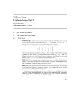
To determine the “best” choice of x, Player 1 analyzes the problem, as follows. . .
2-4
-1
0
1
2
3
x
1
= 0
x
2
= 1
x
1
= 1
x
2
= 0
x
1
= 1/5
3/5
 ✁

✂✄☎✆
✝
Player 2 might do the same thing using probability vector y = (y
1
, y
2
) where

i
y
i
= 1 and y
i
≥ 0 for all i.
-1
0
1
2
3
y
1
= 0
y
2
= 1
y
1
= 1
y
2

= 0
y
1
= 2/5
3/5
 ✁
✂✄☎✆
✝
2-5
If Player 1 adopts mixed strategy (x
1
, x
2
) and Player 2 adopts mixed strategy
(y
1
, y
2
), we obtain an expected payoff of
V = 3x
1
y
1
+ 0(1 − x
1
)y
1
− x
1
(1 − y

1
)
+(1 − x
1
)(1 − y
1
)
= 5x
1
y
1
− y
1
− 2x
1
+ 1
Suppose Player 1 uses x
∗
1
=
1
5
, then
V = 5

1
5

y
1

− y
1
− 2

1
5

+ 1 =
3
5
which doesn’t depend on y! Similarly, suppose Player 2 uses y
∗
1
=
2
5
, then
V = 5x
1

2
5

−

2
5

− 2x
1

+ 1 =
3
5
which doesn’t depend on x!
Eachplayerissolvinga constrained optimizationproblem. For Player 1the problem
is
max{v}
st: +3x
1
+ 0x
2
≥ v
−1x
1
+ 1x
2
≥ v
x
1
+ x
2
= 1
x
i
≥ 0 ∀ i
which can be illustrated as follows:
2-6
-1
0
1

2
3
x
1
= 0
x
2
= 1
x
1
= 1
x
2
= 0
 ✁
✂✄☎✆
✝
v
This problem is equivalent to
max
x
min{(3x
1
+ 0x
2
), (−x
1
+ x
2
)}

For Player 2 the problem is
min{v}
st: +3y
1
− 1y
2
≤ v
+0y
1
+ 1y
2
≤ v
y
1
+ y
2
= 1
y
j
≥ 0 ∀ j
which is equivalent to
min
y
max{(3y
1
− y
2
), (0y
1
+ y

2
)}
We recognize these as dual linear programming problems.
Question 2.4. We now have a way to compute a “spy-proof” mixed strategy for
each player. Modify these two mathematical programming problems to produce
the pure security strategy for each player.
2-7
In general, the players are solving the following pair of dual linear programming
problems:
max{v}
st:

i
a
ij
x
i
≥ v ∀ j

i
x
i
= 1
x
i
≥ 0 ∀ i
and
min{v}
st:


j
a
ij
y
j
≤ v ∀ i

i
y
i
= 1
y
i
≥ 0 ∀ j
Note 2.4. Consider, once again, the example game
A =

3 −1
0 1

If Player 1 (the maximizer) uses mixed strategy (x
1
, (1 − x
1
)), and if Player 2 (the
minimizer) uses mixed strategy (y
1
, (1 − y
1
)) we get

E(x, y) = 5x
1
y
1
− y
1
− 2x
1
+ 1
and letting x
∗
=
1
5
and y
∗
=
2
5
we get E(x
∗
, y) = E(x, y
∗
) =
3
5
for any x and y.
These choices for x
∗
and y

∗
make the expected value independent of the opposing
strategy. So, if Player 1 becomes a minimizer (or if Player 2 becomes a maximizer)
the resulting mixed strategies would be the same!
Note 2.5. Consider the game
A =

1 3
4 2

By “factoring” the expression for E(x, y), we can write
E(x, y) = x
1
y
1
+ 3x
1
(1 − y
1
) + 4(1 − x
1
)y + 2(1 − x
1
)(1 − y
1
)
= −4x
1
y
1

+ x
1
+ 2y
1
+ 2
= −4(x
1
y
1
−
x
1
4
−
y
1
2
+
1
8
) + 2 +
1
2
= −4(x
1
−
1
2
)(y
1

−
1
4
) +
5
2
It’s now easy to see that x
∗
1
=
1
2
, y
∗
1
=
1
4
and v =
5
2
.
2-8
2.1.5 A more formal statement of the problem
Suppose we are given a matrix game A
(m×n)
≡

a
ij


. Each row of A is a pure
strategy for Player 1. Each column of A is a pure strategy for Player 2. The value
of a
ij
is the payoff from Player 1 to Player 2 (it may be negative).
For Player 1 let
V (A) = max
i
min
j
a
ij
For Player 2 let
V (A) = min
j
max
i
a
ij
{Case 1} (Saddle Point Case where V (A) = V (A) = V )
Player 1 can assure himself of getting at least V from Player 2 by playing his
maximin strategy.
{Case 2} (Mixed Strategy Case where V (A) < V (A))
Player 1 uses probability vector
x = (x
1
, . . . , x
m
)


i
x
i
= 1 x
i
≥ 0
Player 2 uses probability vector
y = (y
1
, . . . , y
n
)

j
y
j
= 1 y
j
≥ 0
If Player 1 uses x and Player 2 uses strategy j, the expected payoff is
E(x, j) =

i
x
i
a
ij
= xA
j

where A
j
is column j from matrix A.
If Player 2 uses y and Player 1 uses strategy i, the expected payoff is
E(i, y) =

j
a
ij
y
j
= A
i
y
T
where A
i
is row i from matrix A.
2-9
Combined, if Player 1 uses x and Player 2 uses y, the expected payoff is
E(x, y) =

i

j
x
i
a
ij
y

j
= xAy
T
The players are solving the following pair of dual linear programming prob-
lems:
max{v}
st:

i
a
ij
x
i
≥ v ∀ j

i
x
i
= 1
x
i
≥ 0 ∀ i
and
min{v}
st:

j
a
ij
y

j
≤ v ∀ i

i
y
i
= 1
y
i
≥ 0 ∀ j
The Minimax Theorem (von Neumann, 1928) states that there exists mixed strate-
gies x
∗
and y
∗
for Players 1 and 2 which solve each of the above problems with
equal objective function values.
2.1.6 Proof of the Minimax Theorem
Note 2.6. (From Ba¸sar and Olsder [2]) The theory of finite zero-sum games dates
back to Borel in the early 1920’s whose work on the subject was later translated
into English (Borel, 1953). Borel introduced the notion of a conflicting decision
situation that involves more than one decision maker, and the concepts of pure
and mixed strategies, but he did not really develop a complete theory of zero-sum
games. Borel even conjectured that the Minimax Theorem was false.
It was von Neumann who first came up with a proof of the Minimax Theorem,
and laid down the foundations of game theory as we know it today (von Neumann
1928, 1937).
Wewill provide two proofs of this important theorem. The first proof (Theorem 2.4)
uses only the Separating Hyperplane Theorem. The second proof (Theorem 2.5)
uses the similar, but more powerful, tool of duality from the theory linear program-

ming.
2-10