Tài liệu Bài 3: Gradients and Optimization Methods ppt
Bạn đang xem bản rút gọn của tài liệu. Xem và tải ngay bản đầy đủ của tài liệu tại đây (440.89 KB, 20 trang )
3
Gradients and Optimization
Methods
The main task in the independent component analysis (ICA) problem, formulated in
Chapter 1, is to estimate a separating matrix
W
that will give us the independent
components. It also became clear that
W
cannot generally be solved in closed form,
that is, we cannot write it as some function of the sample or training set, whose value
could be directly evaluated. Instead, the solution method is based on cost functions,
also called objective functions or contrast functions. Solutions
W
to ICA are found
at the minima or maxima of these functions. Several possible ICA cost functions will
be given and discussed in detail in Parts II and III of this book. In general, statistical
estimation is largely based on optimization of cost or objective functions, as will be
seen in Chapter 4.
Minimization of multivariate functions, possibly under some constraints on the
solutions, is the subject of optimization theory. In this chapter, we discuss some
typical iterative optimization algorithms and their properties. Mostly, the algorithms
are based on the gradients of the cost functions. Therefore, vector and matrix
gradients are reviewed first, followed by the most typical ways to solve unconstrained
and constrained optimization problems with gradient-type learning algorithms.
3.1 VECTOR AND MATRIX GRADIENTS
3.1.1 Vector gradient
Consider a scalar valued function
g
of
m
variables
g = g (w
1
:::w
m
)=g (w)
57
Independent Component Analysis. Aapo Hyv
¨
arinen, Juha Karhunen, Erkki Oja
Copyright
2001 John Wiley & Sons, Inc.
ISBNs: 0-471-40540-X (Hardback); 0-471-22131-7 (Electronic)
58
GRADIENTS AND OPTIMIZATION METHODS
where we have used the notation
w =(w
1
:::w
m
)
T
. By convention, we define
w
as a column vector. Assuming the function
g
is differentiable, its vector gradient with
respect to
w
is the
m
-dimensional column vector of partial derivatives
@g
@ w
=
0
B
@
@g
@w
1
.
.
.
@g
@w
m
1
C
A
(3.1)
The notation
@g
@ w
is just shorthand for the gradient; it should be understood that it
does not imply any kind of division by a vector, which is not a well-defined concept.
Another commonly used notation would be
rg
or
r
w
g
.
In some iteration methods, we have also reason to use second-order gradients. We
define the second-order gradient of a function
g
with respect to
w
as
@
2
g
@ w
2
=
0
B
B
@
@
2
g
@w
2
1
:::
@
2
g
@w
1
w
m
.
.
.
.
.
.
@
2
g
@w
m
w
1
:::
@
2
g
@w
2
m
1
C
C
A
(3.2)
This is an
m m
matrix whose elements are second order partial derivatives. It is
called the Hessian matrix of the function
g (w)
. It is easy to see that it is always
symmetric.
These concepts generalize to vector-valued functions; this means an
n
-element
vector
g(w)=
0
B
@
g
1
(w)
.
.
.
g
n
(w)
1
C
A
(3.3)
whose elements
g
i
(w)
are themselves functions of
w
.TheJacobian matrix of
g
with
respect to
w
is
@ g
@ w
=
0
B
@
@g
1
@w
1
:::
@g
n
@w
1
.
.
.
.
.
.
@g
1
@w
m
:::
@g
n
@w
m
1
C
A
(3.4)
Thus the
i
th column of the Jacobian matrix is the gradient vector of
g
i
(w)
with
respect to
w
. The Jacobian matrix is sometimes denoted by
J g
.
For computing the gradients of products and quotients of functions, as well as of
composite functions, the same rules apply as for ordinary functions of one variable.
VECTOR AND MATRIX GRADIENTS
59
Thus
@f (w)g (w)
@ w
=
@f (w)
@ w
g (w)+f (w)
@g(w)
@ w
(3.5)
@f (w)=g (w)
@ w
=
@f (w)
@ w
g (w) f (w)
@g(w)
@ w
]=g
2
(w)
(3.6)
@f (g (w))
@ w
= f
0
(g (w))
@g(w)
@ w
(3.7)
The gradient of the composite function
f (g (w))
can be generalized to any number
of nested functions, giving the same chain rule of differentiation that is valid for
functions of one variable.
3.1.2 Matrix gradient
In many of the algorithms encountered in this book, we have to consider scalar-valued
functions
g
of the elements of an
m n
matrix
W =(w
ij
)
:
g = g (W)=g(w
11
:::w
ij
::: w
mn
)
(3.8)
A typical function of this kind is the determinant of
W
.
Of course, any matrix can be trivially represented as a vector by scanning the
elements row by row into a vector and reindexing. Thus, when considering the
gradient of
g
with respect to the matrix elements, it would suffice to use the notion
of vector gradient reviewed earlier. However, using the separate concept of matrix
gradient gives some advantages in terms of a simplified notation and sometimes
intuitively appealing results.
In analogy with the vector gradient, the matrix gradient means a matrix of the
same size
m n
as matrix
W
, whose
ij
th element is the partial derivative of
g
with
respect to
w
ij
. Formally we can write
@g
@ W
=
0
B
@
@g
@w
11
:::
@g
@w
1n
.
.
.
.
.
.
@g
@w
m1
:::
@g
@w
mn
1
C
A
(3.9)
Again, the notation
@g
@ W
is just shorthand for the matrix gradient.
Let us look next at some examples on vector and matrix gradients. The formulas
presented in these examples will be frequently needed later in this book.
3.1.3 Examples of gradients
Example 3.1 Consider the simple linear functional of
w
, or inner product
g (w)=
m
X
i=1
a
i
w
i
= a
T
w
60
GRADIENTS AND OPTIMIZATION METHODS
where
a =(a
1
:::a
m
)
T
is a constant vector. The gradient is, according to (3.1),
@g
@ w
=
0
B
@
a
1
.
.
.
a
m
1
C
A
(3.10)
which is the vector
a
. We can write
@ a
T
w
@ w
= a
Because the gradient is constant (independent of
w
), the Hessian matrix of
g (w)=
a
T
w
is zero.
Example 3.2 Next consider the quadratic form
g (w)=w
T
Aw =
m
X
i=1
m
X
j =1
w
i
w
j
a
ij
(3.11)
where
A =(a
ij
)
is a square
m m
matrix. We have
@g
@ w
=
0
B
@
P
m
j =1
w
j
a
1j
+
P
m
i=1
w
i
a
i1
.
.
.
P
m
j =1
w
j
a
mj
+
P
m
i=1
w
i
a
im
1
C
A
(3.12)
which is equal to the vector
Aw + A
T
w
.So,
@ w
T
Aw
@ w
= Aw + A
T
w
For symmetric
A
, this becomes
2Aw
.
The second-order gradient or Hessian becomes
@
2
w
T
Aw
@ w
2
=
0
B
@
2a
11
::: a
1m
+ a
m1
.
.
.
.
.
.
a
m1
+ a
1m
::: 2a
mm
1
C
A
(3.13)
which is equal to the matrix
A + A
T
.If
A
is symmetric, then the Hessian of
w
T
Aw
is equal to
2A
.
Example 3.3 For the quadratic form (3.11), we might quite as well take the gradient
with respect to
A
, assuming now that
w
is a constant vector. Then
@ w
T
Aw
@a
ij
= w
i
w
j
.
Compiling this into matrix form, we notice that the matrix gradient is the
m m
matrix
ww
T
.
Example 3.4 In some ICA models, we must compute the matrix gradient of the
determinant of a matrix. The determinant is a scalar function of the matrix elements
VECTOR AND MATRIX GRADIENTS
61
consisting of multiplications and summations, and therefore its partial derivatives are
relatively simple to compute. Let us prove the following: If
W
is an invertible square
m m
matrix whose determinant is denoted
det W
,then
@
@ W
det W =(W
T
)
1
det W:
(3.14)
This is a good example for showing that a compact formula is obtained using the
matrix gradient; if
W
were stacked into a long vector, and only the vector gradient
were used, this result could not be expressed so simply.
Instead of starting from scratch, we employ a well-known result from matrix
algebra (see, e.g., [159]), stating that the inverse of a matrix
W
is obtained as
W
1
=
1
det W
adj
(W)
(3.15)
with adj
(W)
the so-called adjoint of
W
. The adjoint is the matrix
adj
(W)=
0
@
W
11
::: W
n1
W
1n
::: W
nn
1
A
(3.16)
where the scalar numbers
W
ij
are the so-called cofactors. The cofactor
W
ij
is
obtained by first taking the
(n 1) (n 1)
submatrix of
W
that remains when
the
i
th row and
j
th column are removed, then computing the determinant of this
submatrix, and finally multiplying by
(1)
i+j
.
The determinant
det W
can also be expressed in terms of the cofactors:
det W =
n
X
k=1
w
ik
W
ik
(3.17)
Row
i
can be any row, and the result is always the same. In the cofactors
W
ik
, none
of the matrix elements of the
i
th row appear, so the determinant is a linear function
of these elements. Taking now a partial derivative of (3.17) with respect to one of the
elements, say,
w
ij
,gives
@ det W
@w
ij
= W
ij
By definitions (3.9) and (3.16), this implies directly that
@ det W
@ W
=
adj
(W)
T
But adj
(W)
T
is equal to
(det W)(W
T
)
1
by (3.15), so we have shown our result
(3.14).
This also implies that
@ log j det Wj
@ W
=
1
j det Wj
@ j det Wj
@ W
=(W
T
)
1
(3.18)
see (3.15). This is an example of the matrix gradient of a composite function
consisting of the
log
, absolute value, and
det
functions. This result will be needed
when the ICA problem is solved by maximum likelihood estimation in Chapter 9.
62
GRADIENTS AND OPTIMIZATION METHODS
3.1.4 Taylor series expansions of multivariate functions
In deriving some of the gradient type learning algorithms, we have to resort to Taylor
series expansions of multivariate functions. In analogy with the well-known Taylor
series expansion of a function
g (w)
of a scalar variable
w
,
g (w
0
)=g (w)+
dg
dw
(w
0
w)+1=2
d
2
g
dw
2
(w
0
w)
2
+ :::
(3.19)
we can do a similar expansion for a function
g (w)=g (w
1
:::w
m
)
of
m
variables.
We h ave
g (w
0
)=g (w)+(
@g
@ w
)
T
(w
0
w)+1=2(w
0
w)
T
@
2
g
@ w
2
(w
0
w)+:::
(3.20)
where the derivatives are evaluated at the point
w
. The second term is the inner
product of the gradient vector with the vector
w
0
w
, and the third term is a quadratic
form with the symmetric Hessian matrix
@
2
g
@ w
2
. The truncation error depends on the
distance
kw
0
wk
; the distance has to be small, if
g (w
0
)
is approximated using only
the first- and second-order terms.
The same expansion can be made for a scalar function of a matrix variable. The
second order term already becomes complicated because the second order gradient is
a four-dimensional tensor. But we can easily extend the first order term in (3.20), the
inner product of the gradient with the vector
w
0
w
, to the matrix case. Remember
that the vector inner product is defined as
(
@g
@ w
)
T
(w
0
w)=
m
X
i=1
(
@g
@ w
)
i
(w
0
i
w
i
)
For the matrix case, this must become the sum
P
m
i=1
P
m
j =1
(
@g
@ W
)
ij
(w
0
ij
w
ij
):
This
is the sum of the products of corresponding elements, just like in the vectorial inner
product. This can be nicely presented in matrix form when we remember that for any
two matrices, say,
A
and
B
,
trace
(A
T
B)=
m
X
i=1
(A
T
B)
ii
=
m
X
i=1
m
X
j =1
(A)
ij
(B)
ij
with obvious notation. So, we have
g (W
0
)=g (W)+
trace
(
@g
@ W
)
T
(W
0
W)] + :::
(3.21)
for the first two terms in the Taylor series of a function
g
of a matrix variable.
LEARNING RULES FOR UNCONSTRAINED OPTIMIZATION
63
3.2 LEARNING RULES FOR UNCONSTRAINED OPTIMIZATION
3.2.1 Gradient descent
Many of the ICA criteria have the basic form of minimizing a cost function
J (W)
with respect to a parameter matrix
W
, or possibly with respect to one of its columns
w
. In many cases, there are also constraints that restrict the set of possible solutions.
A typical constraint is to require that the solution vector must have a bounded norm,
or the solution matrix has orthonormal columns.
For the unconstrained problem of minimizing a multivariate function, the most
classic approach is steepest descent or gradient descent. Let us consider in more
detail the case when the solution is a vector
w
; the matrix case goes through in a
completely analogous fashion.
In gradient descent, we minimize a function
J (w)
iteratively by starting from
some initial point
w(0)
, computing the gradient of
J (w)
at this point, and then
moving in the direction of the negative gradient or the steepest descent by a suitable
distance. Once there, we repeat the same procedure at the new point, and so on. For
t =1 2:::
we have the update rule
w(t)=w(t 1) (t)
@ J (w)
@ w
j
w=w(t1)
(3.22)
with the gradient taken at the point
w(t 1)
. The parameter
(t)
gives the length of
the step in the negative gradient direction. It is often called the step size or learning
rate. Iteration (3.22) is continued until it converges, which in practice happens when
the Euclidean distance between two consequent solutions
kw(t) w(t 1)k
goes
below some small tolerance level.
If there is no reason to emphasize the time or iteration step, a convenient shorthand
notation will be used throughout this book in presenting update rules of the preceding
type. Denote the difference between the new and old value by
w(t) w(t 1) = w
(3.23)
We can then write the rule (3.22) either as
w =
@ J (w)
@ w
or even shorter as
w /
@ J (w)
@ w
The symbol
/
is read “is proportional to”; it is then understood that the vector on the
left-hand side,
w
, has the same direction as the gradient vector on the right-hand
side, but there is a positive scalar coefficient by which the length can be adjusted. In
the upper version of the update rule, this coefficient is denoted by
. In many cases,
this learning rate can and should in fact be time dependent. Yet a third very convenient
way to write such update rules, in conformity with programming languages, is
w w
@ J (w)
@ w
64
GRADIENTS AND OPTIMIZATION METHODS
where the symbol
means substitution, i.e., the value of the right-hand side is
computed and substituted in
w
.
Geometrically, a gradient descent step as in (3.22) means going downhill. The
graph of
J (w)
is the multidimensional equivalent of mountain terrain, and we are
always moving downwards in the steepest direction. This also immediately shows
the disadvantage of steepest descent: unless the function
J (w)
is very simple and
smooth, steepest descent will lead to the closest local minimum instead of a global
minimum. As such, the method offers no way to escape from a local minimum.
Nonquadratic cost functions may have many local maxima and minima. Therefore,
good initial values are important in initializing the algorithm.
Local minimum
Gradient vector
minimum
Global
Fig. 3.1
Contour plot of a cost function with a local minimum.
As an example, consider the case of Fig. 3.1. A function
J (w)
is shown there as
a contour plot. In the region shown in the figure, there is one local minimum and one
global minimum. From the initial point chosen there, where the gradient vector has
been plotted, it is very likely that the algorithm will converge to the local minimum.
Generally, the speed of convergence can be quite low close to the minimum point,
because the gradient approaches zero there. The speed can be analyzed as follows.
Let us denote by
w
the local or global minimum point where the algorithm will
eventually converge. From (3.22) we have
w(t) w
= w(t 1) w
(t)
@ J (w)
@ w
j
w=w(t1)
(3.24)
Let us expand the gradient vector
@ J (w)
@ w
element by element as a Taylor series around
the point
w
, as explained in Section 3.1.4. Using only the zeroth- and first-order
terms, we have for the
i
th element
@ J (w)
@w
i
j
w=w(t1)
=
@ J (w)
@w
i
j
w=w
+
m
X
j =1
@
2
J (w)
@w
i
w
j
j
w=w
w
j
(t 1) w
j
]+:::