Tài liệu Hard Disk Drive Servo Systems- P5 pdf

188 6 Track Following of a Single-stage Actuator
experimental performance. The above discrete-time PID controller is obtained from
a continuous-time counterpart using the ZOH method with a sampling frequency
of 20 kHz. Once again, we note that the above PID controller is tuned to meet the
requirements on the gain and phase margins, and the design specifications on the
sensitivity and complementary sensitivity functions. Although the PID control has
the simplest structure, its dynamical order, which is 3, is higher than that of the RPT
and CNF controllers. As expected, the complete control input is given by
(6.29)
6.4 Simulation and Implementation Results
In this section we present the simulation and actual implementation results of our de-
signs and their comparison. The following tests are presented: i) the track-following
test of the closed-loop systems, ii) the frequency-domain test including the Bode
and Nyquist plots as well as the plots of the resulting sensitivity and complemen-
tary sensitivity functions, iii) the runout disturbance test, and lastly iv) the PES test.
Our controller was implemented on an open HDD with a sampling rate of 20 kHz.
Closed-loop actuation tests were performed using an LDV to measure the R/W head
position. The resolution used for LDV was 2
l
um/V. This displacement output is then
fed into the DSP, which would then generate the necessary control signal to the VCM
actuator. The actual implementation setup is as depicted in Figure 1.7.
6.4.1 Track-following Test
The simulation result and actual implementation result of the closed-loop responses
for the control systems are, respectively, shown in Figures 6.6 and 6.7. It is noted that
the PID control generates large overshoots in both simulation and implementation,
while the systems with the RPT and CNF control have very little overshoot. We sum-
marize the resulting 5% settling time, which is commonly used in the HDD research
community, in Table 6.1. Clearly, the CNF control gives the best performance in the
time domain compared to those of the other two systems.
Table 6.1. Performances of the track-following controllers

Settling time (ms)
PID control RPT control CNF control
Simulation 3.10 0.95 0.80
Implementation 2.65 1.05 0.85
Please purchase PDF Split-Merge on www.verypdf.com to remove this watermark.
6.4 Simulation and Implementation Results 189
0
0.5
1
1.5
2
2.5
3
3.5
4
4.5
5
0
0.5
1
1.5
Time (ms)
Displacement (μm)
PID (overshoot 41%)
RPT
CNF
(a) Output responses
0
0.5
1

1.5
2
2.5
3
3.5
4
4.5
5
−0.05
0
0.05
0.1
Time (ms)
Input signal to VCM (V)
PID
RPT
CNF
(b) Control signals
Figure 6.6. Simulation result: step responses with PID, RPT and CNF control
Please purchase PDF Split-Merge on www.verypdf.com to remove this watermark.
190 6 Track Following of a Single-stage Actuator
0
0.5
1
1.5
2
2.5
3
3.5
4

4.5
5
0
0.2
0.4
0.6
0.8
1
1.2
1.4
Time (ms)
Displacement (μm)
PID (overshoot 31%)
RPT
CNF
(a) Output responses
0
0.5
1
1.5
2
2.5
3
3.5
4
4.5
5
−0.05
0
0.05

0.1
Time (ms)
Input signal to VCM (V)
PID
RPT
CNF
(b) Control signals
Figure 6.7. Implementation result: step responses with PID, RPT and CNF control
Please purchase PDF Split-Merge on www.verypdf.com to remove this watermark.
6.4 Simulation and Implementation Results 191
We believe that the shortcoming of the PID control is mainly due to its structure,
i.e. it only feeds in the error signal,
, instead of feeding in both and inde-
pendently. We trust that the same problem might be present in other control methods
if the only signal fed is
. The PID control structure might well be as simple as
most researchers and engineers have claimed. However, the RPT controller is even
simpler, but it and the CNF controller have fully utilized all available information
associated with the actual system.
Unfortunately, we could not compare our results with those in the literature. Most
of the references we found in the open literature contained only simulation results
in this regard. Some of the implementation results we found were, however, very
different in nature. For example, Hanselmann and Engelke [18] reported an imple-
mentation result of a disk drive control system design using the LQG approach with a
sampling frequency of 34 kHz. The overall step response in [18] with a higher-order
LQG controller and higher sampling frequency is worse than that of ours.
6.4.2 Frequency-domain Test
For practical consideration, it is important and necessary to examine the frequency-
domain properties of control system design, which include the results of gain and
phase margins and the plots of sensitivity and complementary sensitivity functions.

Traditionally, gain and phase margins can be obtained through the Bode plot of the
open-loop transfer function comprising the given plant and the controller. However,
for the HDD system considered in our design, which has additional high-frequency
resonance modes, the corresponding Bode plots might have more than one gain
and/or phase crossover frequencies. Thus, it is important to verify the stability mar-
gins obtained from the associated Nyquist plots. Figures 6.8 to 6.13, respectively,
show the Bode plot, the Nyquist plot, and the sensitivity and complementary sen-
sitivity functions, as well as the closed-loop transfer functions (from the reference
input
to the controlled output ) of the resulting control systems. For the
CNF design, which is a nonlinear controller, its frequency-domain functions are cal-
culated at the steady-state situation for which the nonlinear gain function
has
approached its final constant value. The results show that all these designs meet the
frequency-domain specifications and have about the same closed-loop bandwidth.
6.4.3 Runout Disturbance Test
Although we do not consider the effects of runout disturbances in our problem for-
mulation, it turns out that our controllers are capable of rejecting the repeatable
runout disturbances, which are mainly due to the imperfectness of the data tracks
and the spindle motor speeds, and commonly have frequencies at the multiples of
the spindle speed, which is about
Hz. We simulate these runout effects by inject-
ing a sinusoidal signal into the measurement output, i.e. the new measurement output
is the sum of the actuator output and the runout disturbance. Figure 6.14 shows the
implementation result of the output responses of the overall control system compris-
ing the tenth-order model of the VCM actuator model and the controllers together
Please purchase PDF Split-Merge on www.verypdf.com to remove this watermark.
192 6 Track Following of a Single-stage Actuator
10
0

10
1
10
2
10
3
10
4
10
5
−200
−150
−100
−50
0
50
100
Frequency (Hz)
Magnitude (dB)
10
0
10
1
10
2
10
3
10
4
10

5
−700
−600
−500
−400
−300
−200
−100
Frequency (Hz)
Phase (deg)
GM = 16.4 dB
PM = 46.5
°
(a) Bode plot
−1
−0.8
−0.6
−0.4
−0.2
0
−1
−0.8
−0.6
−0.4
−0.2
0
0.2
0.4
0.6
0.8

1
0 dB
−20 dB
−10 dB
−6 dB
−4 dB
−2 dB
20 dB
10 dB
6 dB
4 dB
2 dB
Real axis
Imaginary axis
(b) Nyquist plot
Figure 6.8. Bode and Nyquist plots of the PID control system
Please purchase PDF Split-Merge on www.verypdf.com to remove this watermark.
6.4 Simulation and Implementation Results 193
10
0
10
1
10
2
10
3
10
4
10
5

−200
−150
−100
−50
0
50
100
Frequency (Hz)
Magnitude (dB)
10
0
10
1
10
2
10
3
10
4
10
5
−600
−500
−400
−300
−200
−100
Frequency (Hz)
Phase (deg)
GM = 11.7 dB

PM = 35.5
°
(a) Bode plot
−1
−0.8
−0.6
−0.4
−0.2
0
0.2
−0.8
−0.6
−0.4
−0.2
0
0.2
0.4
0.6
0.8
0 dB
−20 dB
−10 dB
−6 dB
−4 dB−2 dB
20 dB
10 dB
6 dB
4 dB 2 dB
Real axis
Imaginary axis

(b) Nyquist plot
Figure 6.9. Bode and Nyquist plots of the RPT control system
Please purchase PDF Split-Merge on www.verypdf.com to remove this watermark.
194 6 Track Following of a Single-stage Actuator
10
0
10
1
10
2
10
3
10
4
10
5
−200
−150
−100
−50
0
50
100
Frequency (Hz)
Magnitude (dB)
10
0
10
1
10

2
10
3
10
4
10
5
−600
−500
−400
−300
−200
−100
Frequency (Hz)
Phase (deg)
GM = 8.6 dB
PM = 40
°
(a) Bode plot
−1
−0.8
−0.6
−0.4
−0.2
0
0.2
−1
−0.8
−0.6
−0.4

−0.2
0
0.2
0.4
0.6
0.8
1
0 dB
−20 dB
−10 dB
−6 dB
−4 dB
−2 dB
20 dB
10 dB
6 dB
4 dB
2 dB
Real axis
Imaginary axis
(b) Nyquist plot
Figure 6.10. Bode and Nyquist plots of the CNF control system
Please purchase PDF Split-Merge on www.verypdf.com to remove this watermark.
6.4 Simulation and Implementation Results 195
10
0
10
1
10
2

10
3
10
4
10
5
−120
−100
−80
−60
−40
−20
0
Frequency (Hz)
Magnitude (dB)
T function (max. 3.1 dB)
S function (max. 3.1 dB)
(a) Sensitivity and complementary sensitivity functions
10
0
10
1
10
2
10
3
10
4
10
5

−200
−150
−100
−50
0
Frequency (Hz)
Magnitude (dB)
10
0
10
1
10
2
10
3
10
4
10
5
−800
−600
−400
−200
0
Frequency (Hz)
Phase (deg)
BW = 514 Hz
(b) Closed-loop response
Figure 6.11. Sensitivity functions and closed-loop transfer function of the PID control system
Please purchase PDF Split-Merge on www.verypdf.com to remove this watermark.

196 6 Track Following of a Single-stage Actuator
10
0
10
1
10
2
10
3
10
4
10
5
−120
−100
−80
−60
−40
−20
0
Frequency (Hz)
Magnitude (dB)
T function (max. 4.7 dB)
S function (max. 5.2 dB)
(a) Sensitivity and complementary sensitivity functions
10
0
10
1
10

2
10
3
10
4
10
5
−200
−150
−100
−50
0
Frequency (Hz)
Magnitude (dB)
10
0
10
1
10
2
10
3
10
4
10
5
−600
−500
−400
−300

−200
−100
0
Frequency (Hz)
Phase (deg)
BW = 553 Hz
(b) Closed-loop response
Figure 6.12. Sensitivity functions and closed-loop transfer function of the RPT control system
Please purchase PDF Split-Merge on www.verypdf.com to remove this watermark.
6.4 Simulation and Implementation Results 197
10
0
10
1
10
2
10
3
10
4
10
5
−120
−100
−80
−60
−40
−20
0
Frequency (Hz)

Magnitude (dB)
T function (max. 3.6 dB)
S function (max. 4.9 dB)
(a) Sensitivity and complementary sensitivity functions
10
0
10
1
10
2
10
3
10
4
10
5
−200
−150
−100
−50
0
Frequency (Hz)
Magnitude (dB)
10
0
10
1
10
2
10

3
10
4
10
5
−600
−500
−400
−300
−200
−100
0
Frequency (Hz)
Phase (deg)
BW = 576 Hz
(b) Closed-loop response
Figure 6.13. Sensitivity functions and closed-loop transfer function of the CNF control system
Please purchase PDF Split-Merge on www.verypdf.com to remove this watermark.
198 6 Track Following of a Single-stage Actuator
with a fictitious runout disturbance injection
(6.30)
and a zero reference
. The result shows that the RPT and CNF controllers again
have better performance and the effects of such a disturbance on the overall response
under CNF control are minimal. A more comprehensive test on runout disturbances,
i.e. the position error signal (PES) test on the actual system will be presented in the
next section.
0
10
20

30
40
50
60
70
80
90
100
0.3
0.4
0.5
0.6
RRO disturbance (μm)
0
10
20
30
40
50
60
70
80
90
100
−0.05
0
0.05
Error (μm)
0
10

20
30
40
50
60
70
80
90
100
−0.05
0
0.05
Error (μm)
0
10
20
30
40
50
60
70
80
90
100
−0.05
0
0.05
Error (μm)
Time (ms)
PID

RPT
CNF
Figure 6.14. Closed-loop output responses due to a runout disturbance
6.4.4 Position Error Signal Test
The disturbances in a real HDD are usually considered as a lumped disturbance at the
plant output, also known as runouts. Repeatable runouts (RROs) and nonrepeatable
runouts (NRROs) are the major sources of track-following errors. RROs are caused
by the rotation of the spindle motor and consists of frequencies that are multiples of
the spindle frequency. NRROs can be perceived as coming from three main sources:
vibration shocks, mechanical disturbance and electrical noise. Static force due to
Please purchase PDF Split-Merge on www.verypdf.com to remove this watermark.
6.4 Simulation and Implementation Results 199
flex cable bias, pivot-bearing friction and windage are all components of the vibra-
tion shock disturbance. Mechanical disturbances include spindle motor variations,
disk flutter and slider vibrations. Electrical noises include quantization errors, media
noise, servo demodulator noise and power amplifier noise. NRROs are usually ran-
dom and unpredictable by nature, unlike repeatable runouts. They are also of a lower
magnitude (see, e.g., [1]). A perfect servo system for HDDs has to reject both the
RROs and NRROs.
In our experiment, we have simplified the system somewhat by removing many
sources of disturbances, especially that of the spinning magnetic disk. Therefore, we
actually have to add the runouts and other disturbances into the system manually.
Based on previous experiments, we know that the runouts in real disk drives are
composed mainly of RROs, which are basically sinusoidal with a frequency of about
55 Hz, equivalent to the spin rate of the spindle motor. By manually adding this
“noise” to the output while keeping the reference signal at zero, we can then read
off the subsequent position signal as the expected PES in the presence of runouts.
For actual drives, prewritten PES data might be estimated at high sampling rates
using servo sector measurements (see, for example, [141]). In disk drive applications,
the variation in the position of the R/W head from the center of the track during

track following, which can be directly read off as the PES, is very important. Track-
following servo systems have to ensure that the PES is kept to a minimum. Having
deviations that are above the tolerance of the disk drive would result in too many read
or write errors, making the disk drive unusable. A suitable measure is the standard
deviation of the readings,
. A useful guideline is to make the value less
than
of the track pitch, which is about
l
um for a track density of 25 kTPI.
Figure 6.15 shows the histograms of the tracking errors of the respective control
systems under the disturbance of the runouts. The
values of the PES test are
summarized in Table 6.2. Again, the CNF control yields the best performance in the
PES test.
Table 6.2. The values of the PES test
PID control RPT control CNF control
3 (
l
um) 0.0615 0.0375 0.0288
In conclusion, the RPT and CNF controllers have much better performance in
track following and in the PES tests compared with that of the PID controller. We
note that the results can be further improved if we used a better VCM actuator and
arm assembly (such as those used in minidrives and microdrives) with a higher reso-
nance frequency. We will carry out a detailed study on the servo system of a micro-
drive later in Chapter 9.
Please purchase PDF Split-Merge on www.verypdf.com to remove this watermark.
200 6 Track Following of a Single-stage Actuator
−0.1
0

0.1
0
500
1000
1500
2000
2500
3000
3500
4000
Points
Error (μm)
−0.1
0
0.1
0
500
1000
1500
2000
2500
3000
3500
4000
Error (μm)
−0.1
0
0.1
0
500

1000
1500
2000
2500
3000
3500
4000
Error (μm)
PID
RPT
CNF
Figure 6.15. Implementation result: histograms of the PES tests
Please purchase PDF Split-Merge on www.verypdf.com to remove this watermark.
7
Track Seeking of a Single-stage Actuator
7.1 Introduction
In this chapter, we proceed to design track-seeking controllers for a single-stage actu-
ated HDD that would give high-speed seeking performance. We utilize the nonlinear
control techniques reported in Chapters 4 and 5 as well as the linear techniques re-
ported in Chapter 3 to carry out the design of three different types of track-seeking
controllers for a Maxtor HDD with a single VCM actuator. More specifically, we
design the servo systems using the conventional PTOS approach, the CNF control
technique, and the MSC system with PTOS and RPT controllers.
As in Chapter 6, a Maxtor (Model 51536U3) HDD is used to implement our
design. The actual frequency response and the identified model are given Figure 6.1.
The frequency-domain model has been identified earlier in Chapter 6 and is given
in Equations 6.4–6.8. The same notch filter as in Equation 6.9 is again utilized for
track seeking. With such a formulation, it is safe to approximate the VCM actuator
model with the notch filter as a double integrator with an appropriate gain. Such an
approximation simplifies the overall design procedure a great deal. Most importantly,

it works very well. However, in order to make our design more realistic, all our
simulation results are done using the tenth-order model. The final implementation is,
of course, to be carried out on the actual system.
The following state-space model is then used throughout our design of track-
seeking controllers:
sat (7.1)
where
and are, respectively, the position of the VCM actuator head in microm-
eters and velocity in micrometers per second, and
is the control input in volts. In
general, the velocity of the VCM actuator in the actual system is not available, and
thus
is the only measurable state variable. For this particular system, the controlled
output is also the measurement output, i.e.
(7.2)
Please purchase PDF Split-Merge on www.verypdf.com to remove this watermark.
202 7 Track Seeking of a Single-stage Actuator
Our objective is to design a servo controller that meets the following physical con-
straints and design specifications:
1. the control input does not exceed
V owing to physical constraints on the
actual VCM actuator;
2. the overshoot and undershoot of track seeking are kept to less than 0.5
l
um, the
limit of our measurement device for large displacement. As such, the settling
time used in this chapter is defined as the time taken for the R/W head to reach
the
l
um of the target track from its initial point.

3. the gain margin and phase margin of the overall design are, respectively, greater
than 6 dB and
.
As mentioned earlier, three different approaches, namely the PTOS method, the
MSC method and the CNF method, are presented in the following to design appro-
priate servo systems for the given HDD. We carry out control system design for each
method first. All simulation and implementation results, as well as their comparison
are to be discussed in the last section.
7.2 Track Seeking with PTOS Control
We present in this section the design and implementation of an HDD servo system
using the PTOS approach (see Chapter 4). The first step is to find the state feedback
gains
and in the PTOS control law based on the design specifications. To get
specifications in terms of required closed-loop poles we need the natural frequency
and the damping ratio . Let us choose the natural frequency to be rad/s,
i.e. 500 Hz, and the damping factor to be 0.7255 so as to have an acceleration dis-
count factor
of 0.95, which yields a reasonably good performance for seek lengths
up to 300
l
um. It follows from Equation 4.32 that a PTOS control law with such a dis-
count factor only increases the total tracking time by about 1.6% from that required
in the TOC. Clearly, the performance of the PTOS control is pushed very closely
to its limit, the TOC. Interested readers are referred to [30, 142, 143] for detailed
information on the selection of these parameters. Note that the relation between the
damping ratio
and the acceleration discount factor in PTOS control law is given by
(see [30])
(7.3)
Then, the corresponding

-plane closed-loop poles are
(7.4)
Using the m-function acker in MATLAB
R
, we obtain the following feedback gains
and (7.5)
and the length of the linear region in PTOS can be found from Equation 4.31 and
is given by
l
um. Thus, the PTOS control law for our disk drive is as
follows:
Please purchase PDF Split-Merge on www.verypdf.com to remove this watermark.
7.3 Track-seeking with MSC 203
P
sat (7.6)
where
with being the target reference, and
for
sgn for
(7.7)
with
(7.8)
and
(7.9)
The advantage of this control scheme is that it is quite simple to understand. The
implementation of such a controller requires an estimation of the VCM actuator ve-
locity (with the estimator pole being placed at
). More precisely, the following
velocity estimator is used:
P

(7.10)
and
(7.11)
In the actual simulation and implementation of the PTOS controller of Equation 7.6,
is replaced with of Equation 7.11 and
P
(7.12)
where
is as given in Equation 6.9. The simulation and implementation
results of the above design will be given later in Section 7.5.
7.3 Track-seeking with MSC
In this section, we apply the MSC method of Chapter 4 to the disk drive given earlier.
The MSC scheme uses the proximate time-optimal controller in the track-seeking
mode, and the RPT controller in the track-following mode. We note that in MSC,
initially, the plant is controlled by the seeking controller and at the end of the seek-
ing mode a switch changes it to a track-following controller. In [127], the mode
switching was done after finding the optimal mode-switching conditions such that
the impact of the initial values on settling performance was minimized. But the im-
pact of the resulting control signal on the resonance modes was not considered. It
has been shown [74, 106] that the RPT controller is independent of these initial val-
ues. The optimal mode-switching conditions in our scheme can just be set such that
the control signal is small enough so as not to excite the resonance vibrations. The
Please purchase PDF Split-Merge on www.verypdf.com to remove this watermark.
204 7 Track Seeking of a Single-stage Actuator
problem of unmodeled mechanical resonance can be treated more rigorously either
by minimizing the jerk as defined by
as reported in [144] or by using a
method developed in the frequency domain in [145]. However, by utilizing the fea-
tures of RPT control, such as it works for a wide range of resonance frequencies (see
Chapter 6), the mode-switching conditions can be determined in a very simple way

(see Chapter 4).
We now move to present an MSC controller for the HDD with a single VCM
actuator. The control law in track-seeking mode (here we label its control signal as
P
) is given in Equation 7.6, as this mode uses the PTOS control. The control law in
the track-following mode, i.e. the reduced-order measurement feedback RPT control
law, is given by
RC RC R RC RC
(7.13)
with
being the target reference and
RC
RC
RC
RC
(7.14)
Next we find the mode-switching conditions as defined in Equation 4.62. Using
the RPT controller parameters, and following the results of Chapter 4, the mode-
switching conditions can be determined as
l
um
l
um and
l
um/s. We select the MSC law
P
R
(7.15)
in which
P

is as given in Equation 7.6 and is chosen such that
l
um and
l
um/s (7.16)
As in the PTOS case, the actual control signal is generated by
(7.17)
The overall closed-loop system comprising the given VCM actuated HDD and the
MSC control law is asymptotically stable. For easy comparison, the simulation and
implementation of the overall system with the MSC control law will again be pre-
sented in Section 7.5.
Please purchase PDF Split-Merge on www.verypdf.com to remove this watermark.
7.4 Track Seeking with CNF Control 205
7.4 Track Seeking with CNF Control
We now move to the design of a reduced-order continuous-time composite nonlin-
ear control law as given by Equations 5.79 and 5.80 for the commercial hard disk
model shown in Figure 6.1. As the CNF control law depends on the size of the step
command input, we derive, for our HDD model given in Equation 7.1, the following
parameterized state feedback gain
:
(7.18)
which places the eigenvalues of
exactly at and
. The latter is the pole associated with the integration dynamics. Following
the design procedure given in Chapter 5 and the physical properties of the given
system, for
l
um, which is to be used in the next section for simulation and
implementation, we choose a damping ratio of
and Hz, which

corresponds roughly to the normal working frequency range of the linear part of the
CNF control law with
. Selecting , and
(7.19)
we obtain
(7.20)
and a reduced-order CNF control law as follows:
(7.21)
with
being the target reference,
(7.22)
and
sat (7.23)
where
(7.24)
(7.25)
and
Please purchase PDF Split-Merge on www.verypdf.com to remove this watermark.
206 7 Track Seeking of a Single-stage Actuator
(7.26)
Again, the actual control signal is generated as follows:
(7.27)
Note that in both simulation and implementation, the initial condition of
is set to
zero at
and reset to zero when the R/W head of the actuator reaches the point
that is 2
l
um from the target to reinforce the integration action. Again, the simulation
and implementation results of the servo system with the CNF control law will be

presented in the next section for an easy comparison.
7.5 Simulation and Implementation Results
Now, we are ready to present the simulation and implementation results for all three
servo systems discussed in the previous sections and do a full-scale comparison on
the performances of these methods. In particular, we study the following tests:
1. track-seeking test;
2. frequency-domain test;
3. runout disturbance test; and
4. PES test.
All simulation results presented in this section have been obtained using Simulink
R
in MATLAB
R
and all implementation results are carried out using our own exper-
imental setup as described in Chapter 1. The sampling frequency for actual imple-
mentation is chosen as
kHz. Here, we note that all our controllers are discretized
using the ZOH technique.
7.5.1 Track-seeking Test
In our simulation and implementation, we use a track pitch of 1
l
um for the HDD. In
what follows, we present results for a track seek length of 300
l
um. Unfortunately,
owing to the capacity of the LDV that has been used to measure the displacement
of the R/W head of the VCM actuator, the absolute errors of our implementation
results given below are 0.5
l
um. As such, the settling time for both implementation

and simulation results is defined as the total time required for the R/W head to move
from its initial position to the entrance of the region of the final target with plus and
minus the absolute error. This is the best we can do with our current experimental
setup. Nonetheless, the results we obtain here are sufficient to illustrate our design
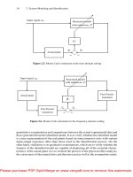
ideas and philosophy. The simulation and implementation results of the track-seeking
performances of the obtained servo systems are, respectively, shown in Figures 7.1
and 7.2. We summarize the overall results on settling times in Table 7.1.
Clearly, the simulation and implementation results show that the servo system
with the CNF controller has the best performance. We believe that this is due to the
fact that the CNF control law unifies the nonlinear and linear components without
switching, whereas the other two servo systems involve switching elements between
the nonlinear and linear parts, which degrades the overall performance.
Please purchase PDF Split-Merge on www.verypdf.com to remove this watermark.
7.5 Simulation and Implementation Results 207
0
1
2
3
4
5
6
0
50
100
150
200
250
300
Time (ms)
Displacement (μm)

MSC
PTOS
CNF
2.8
3
3.2
3.4
3.6
3.8
4
4.2
4.4
299
299.5
300
300.5
Time (ms)
Displacement (μm)
MSC
PTOS
CNF
(a) Output responses
0
1
2
3
4
5
6
−3

−2
−1
0
1
2
3
Time (ms)
Input signal to VCM (V)
MSC
PTOS
CNF
(b) Control signals
Figure 7.1. Simulation result: response and control of the track-seeking systems
Please purchase PDF Split-Merge on www.verypdf.com to remove this watermark.