Tài liệu Hard Disk Drive Servo Systems- P3 ppt

3.6 Robust and Perfect Tracking Control 85
We also assume that the pair is stabilizable and is detectable. For
future reference, we define
P
and
Q
to be the subsystems characterized by the ma-
trix quadruples
and respectively. Given the external
disturbance
, , and any reference signal vector , the RPT
problem for the discrete-time system in Equation 3.238 is to find a parameterized
dynamic measurement feedback control law of the following form:
(3.239)
such that, when the controller in Equation 3.239 is applied to the system in Equation
3.238,
1. there exists an
such that the resulting closed-loop system with and
is asymptotically stable for all ; and
2. let
be the closed-loop controlled output response and let be the
resulting tracking error, i.e.
. Then, for any initial con-
dition of the state,
, as .
It has been shown by Chen [74] that the above RPT problem is solvable for the
system in Equation 3.238 if and only if the following conditions hold:
1.
is stabilizable and is detectable;
2.
, where ;

3.
P
is right invertible and of minimum phase with no infinite zeros;
4. Ker
Im .
It turns out that the control laws, which solve the RPT for the given plant in
Equation 3.238 under the solvability conditions, need not be parameterized by any
tuning parameter. Thus, Equation 3.239 can be replaced by
(3.240)
and, furthermore, the resulting tracking error
can be made identically zero for
all
.
Assume that all the solvability conditions are satisfied. We present in the follow-
ing solutions to the discrete-time RPT problem.
i. State Feedback Case. When all states of the plant are measured for feedback, the
problem can be solved by a static control law. We construct in this subsection a state
feedback control law,
(3.241)
that solves the RPT problem for the system in Equation 3.238. We have the following
algorithm.
S
TEP
3.6.
D
.
S
.1: this step transforms the subsystem from to of the given system
in Equation 3.238 into the special coordinate basis of Theorem 3.1, i.e. finds
Please purchase PDF Split-Merge on www.verypdf.com to remove this watermark.

86 3 Linear Systems and Control
nonsingular state, input and output transformations , and to put it into
the structural form of Theorem 3.1 as well as in the compact form of Equations
3.20 to 3.23, i.e.
(3.242)
(3.243)
(3.244)
(3.245)
S
TEP
3.6.
D
.
S
.2: choose an appropriate dimensional matrix such that
(3.246)
is asymptotically stable. The existence of such an
is guaranteed by the prop-
erty that
is completely controllable.
S
TEP
3.6.
D
.
S
.3: finally, we let
and (3.247)
This ends the constructive algorithm.
We have the following result.

Theorem 3.25. Consider the given discrete-time system in Equation 3.238 with any
external disturbance
and any initial condition . Assume that all its states
are measured for feedback, i.e.
and , and the solvability conditions
for the RPT problem hold. Then, for any reference signal
, the proposed RPT
problem is solved by the control law of Equation 3.241 with
and as given in
Equation 3.247.
ii. Measurement Feedback Case. Without loss of generality, we assume throughout
this subsection that matrix
. If it is nonzero, it can always be washed out by
the following preoutput feedback
It turns out that, for discrete-time
systems, the full-order observer-based control law is not capable of achieving the
RPT performance, because there is a delay of one step in the observer itself. Thus,
we focus on the construction of a reduced-order measurement feedback control law
to solve the RPT problem. For simplicity of presentation, we assume that matrices
and have already been transformed into the following forms,
and (3.248)
where
is of full row rank. Before we present a step-by-step algorithm to con-
struct a reduced-order measurement feedback controller, we first partition the fol-
lowing system
Please purchase PDF Split-Merge on www.verypdf.com to remove this watermark.
3.6 Robust and Perfect Tracking Control 87
(3.249)
in conformity with the structures of
and in Equation 3.248, i.e.

where and . Obviously, is directly
available and hence need not be estimated. Next, let
QR
be characterized by
R R R R
It is straightforward to verify that
QR
is right invertible with no finite and infinite
zeros. Moreover,
R R
is detectable if and only if is detectable. We are
ready to present the following algorithm.
S
TEP
3.6.
D
.
R
.1: for the given system in Equation 3.238, we again assume that
all the state variables of the given system are measurable and then follow Steps
3.6.
D
.
S
.1 to 3.6.
D
.
S
.3 of the algorithm of the previous subsection to construct
gain matrices

and . We also partition in conformity with and as
follows:
(3.250)
S
TEP
3.6.
D
.
R
.2: let
R
be an appropriate dimensional constant matrix such that
the eigenvalues of
R R R R R
(3.251)
are all in
. This can be done because
R R
is detectable.
S
TEP
3.6.
D
.
R
.3: let
R R R R R R R
(3.252)
R R R R
R R R

R
(3.253)
and
R
(3.254)
Please purchase PDF Split-Merge on www.verypdf.com to remove this watermark.
88 3 Linear Systems and Control
S
TEP
3.6.
D
.
R
.4: finally, we obtain the following reduced-order measurement feed-
back control law:
(3.255)
This completes the algorithm.
Theorem 3.26. Consider the given system in Equation 3.238 with any external dis-
turbance
and any initial condition . Assume that the solvability conditions
for the RPT problem hold. Then, for any reference signal
, the proposed RPT
problem is solved by the reduced-order measurement feedback control laws of Equa-
tion 3.255.
3.7 Loop Transfer Recovery Technique
Another popular design methodology for multivariable systems, which is based on
the ‘loop shaping’ concept, is linear quadratic Gaussian (LQG) with loop transfer
recovery (LTR). It involves two separate designs of a state feedback controller and
an observer or an estimator. The exact design procedure depends on the point where
the unstructured uncertainties are modeled and where the loop is broken to evaluate

the open-loop transfer matrices. Commonly, either the input point or the output point
of the plant is taken as such a point. We focus on the case when the loop is broken
at the input point of the plant. The required results for the output point can be easily
obtained by appropriate dualization. Thus, in the two-step procedure of LQG/LTR,
the first step of design involves loop shaping by a state feedback design to obtain
an appropriate loop transfer function, called the target loop transfer function. Such
a loop shaping is an engineering art and often involves the use of linear quadratic
regulator (LQR) design, in which the cost matrices are used as free design param-
eters to generate the target loop transfer function, and thus the desired sensitivity
and complementary sensitivity functions. However, when such a feedback design is
implemented via an observer-based controller (or Kalman filter) that uses only the
measurement feedback, the loop transfer function obtained, in general, is not the
same as the target loop transfer function, unless proper care is taken in designing the
observers. This is when the second step of LQG/LTR design philosophy comes into
the picture. In this step, the required observer design is attempted so as to recover the
loop transfer function of the full state feedback controller. This second step is known
as LTR.
The topic of LTR was heavily studied in the 1980s. Major contributions came
from [109–119]. We present in the following the methods of LTR design at both the
input point and output point of the given plant.
3.7.1 LTR at Input Point
It turns out that it is very simple to formulate the LTR design technique for both
continuous- and discrete-time systems into a single framework. Thus, we do it in one
Please purchase PDF Split-Merge on www.verypdf.com to remove this watermark.
3.7 Loop Transfer Recovery Technique 89
shot. Let us consider a linear time-invariant multivariable system characterized by
(3.256)
where
,if is a continuous-time system, or ,if
is a discrete-time system. Similarly, , and are the state,

input and output of
. They represent, respectively, , and if the given
system is of continuous-time, or represent, respectively,
, and if is
of discrete-time. Without loss of any generality, we assume throughout this section
that both
and are of full rank. The transfer function of is then
given by
(3.257)
where
, the Laplace transform operator, if is of continuous-time, or ,
the
-transform operator, if is of discrete-time.
As mentioned earlier, there are two steps involved in LQG/LTR design. In the
first step, we assume that all state variables of the system in Equation 3.256 are
available and design a full state feedback control law
(3.258)
such that
1. the closed-loop system is asymptotically stable, and
2. the open-loop transfer function when the loop is broken at the input point of the
given system, i.e.
(3.259)
meets some frequency-dependent specifications.
Arriving at an appropriate value for
is concerned with the issue of loop shaping,
which often includes the use of LQR design in which the cost matrices are used as
free design parameters to generate
that satisfies the given specifications.
To be more specific, if
is a continuous-time system, the target loop transfer

function
can be generated by minimizing the following cost function:
C
(3.260)
where
and are free design parameters provided that has
no unobservable modes on the imaginary axis. The solution to the above problem is
given by
(3.261)
where
is the stabilizing solution of the following algebraic Riccati equation
(ARE):
(3.262)
Please purchase PDF Split-Merge on www.verypdf.com to remove this watermark.
90 3 Linear Systems and Control
It is known in the literature that a target loop transfer function with given as
in Equation 3.261 has a phase margin greater than
and an infinite gain margin.
Similarly, if
is a discrete-time system, we can generate a target loop transfer
function
by minimizing
D
(3.263)
where
and are free design parameters provided that has no
unobservable modes on the unit circle.
(3.264)
where
is the stabilizing solution of the following ARE:

(3.265)
Unfortunately, there are no guaranteed phase and gain margins for the target loop
transfer function
resulting from the discrete-time linear quadratic regulator.
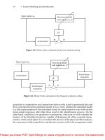
Figure 3.5. Plant-controller closed-loop configuration
Generally, it is unreasonable to assume that all the state variables of a given
system can be measured. Thus, we have to implement the control law obtained in the
first step by a measurement feedback controller. The technique of LTR is to design
an appropriate measurement feedback control (see Figure 3.5) such that the resulting
system is asymptotically stable and the achieved open-loop transfer function
from to is either exactly or approximately matched with the target loop transfer
function
obtained in the first step. In this way, all the nice properties associated
with the target loop transfer function can be recovered by the measurement feedback
controller. This is the so-called LTR design.
It is simple to observe that the achieved open-loop transfer function in the con-
figuration of Figure 3.5 is given by
(3.266)
Please purchase PDF Split-Merge on www.verypdf.com to remove this watermark.
3.7 Loop Transfer Recovery Technique 91
Let us define recovery error as
(3.267)
The LTR technique is to design an appropriate stabilizing
such that the recov-
ery error
is either identically zero or small in a certain sense. As usual, two
commonly used structures for
are: 1) the full-order observer-based controller,
and 2) the reduced-order observer-based controller.
i. Full-order Observer-based Controller. The dynamic equations of a full-order

observer-based controller are well known and are given by
(3.268)
where
is the full-order observer gain matrix and is the only free design parameter.
It is chosen so that
is asymptotically stable. The transfer function of the
full-order observer-based control is given by
(3.269)
It has been shown [110, 117] that the recovery error resulting from the full-order
observer-based controller can be expressed as
(3.270)
where
(3.271)
Obviously, in order to render
to be zero or small, one has to design an observer
gain
such that , or equivalently , is zero or small (in a certain sense).
Defining an auxiliary system,
(3.272)
with a state feedback control law,
(3.273)
It is straightforward to verify that the closed-loop transfer matrix from
to of
the above system is equivalent to
. As such, any of the methods presented in
Sections 3.4 and 3.5 for
and optimal control can be utilized to find to
minimize either the
-norm or -norm of . In particular,
1. if the given plant

is a continuous-time system and if is left invertible and of
minimum phase,
2. if the given plant
is a discrete-time system and if is left invertible and of
minimum phase with no infinite zeros,
Please purchase PDF Split-Merge on www.verypdf.com to remove this watermark.
92 3 Linear Systems and Control
then either the -norm or -norm of can be made arbitrarily small, and
hence LTR can be achieved. If these conditions are not satisfied, the target loop
transfer function
, in general, cannot be fully recovered!
For the case when the target loop transfer function can be approximately recov-
ered, the following full-order Chen–Saberi–Sannuti (CSS) architecture-based control
law (see [111, 117]),
(3.274)
which has a resulting recovery error,
(3.275)
can be utilized to recover the target loop transfer function as well. In fact, when
the same gain matrix
is used, the full-order CSS architecture-based controller
would yield a much better recovery compared to that of the full order observer-based
controller.
ii. Reduced-order Observer-based Controller. For simplicity, we assume that
and have already been transformed into the form
and (3.276)
where
is of full row rank. Then, the dynamic equations of can be partitioned
as follows:
(3.277)
where

is readily accessible. Let
(3.278)
and the reduced-order observer gain matrix
be such that is asymptot-
ically stable. Next, we partition
(3.279)
in conformity with the partitions of
and , respectively. Then,
define
(3.280)
The reduced-order observer-based controller is given by
(3.281)
Please purchase PDF Split-Merge on www.verypdf.com to remove this watermark.
3.7 Loop Transfer Recovery Technique 93
It is again reported in [110, 117] that the recovery error resulting from the reduced-
order observer-based controller can be expressed as
(3.282)
where
(3.283)
Thus, making
zero or small is equivalent to designing a reduced-order observer
gain
such that , or equivalently , is zero or small. Following the same
idea as in the full-order case, we define an auxiliary system
(3.284)
with a state feedback control law,
(3.285)
Obviously, the closed-loop transfer matrix from
to of the above system is equiv-
alent to

. Hence, the methods of Sections 3.4 and 3.5 for and optimal
control again can be used to find
to minimize either the -norm or -norm of
. In particular, for the case when satisfies Condition 1 (for continuous-time
systems) or Condition 2 (for discrete-time systems) stated in the full-order case, the
target loop can be either exactly or approximately recovered. In fact, in this case, the
following reduced-order CSS architecture-based controller
(3.286)
which has a resulting recovery error,
(3.287)
can also be used to recover the given target loop transfer function. Again, when the
same
is used, the reduced-order CSS architecture-based controller would yield a
better recovery compared to that of the reduced-order observer-based controller (see
[111, 117]).
3.7.2 LTR at Output Point
For the case when uncertainties of the given plant are modeled at the output point,
the following dualization procedure can be used to find appropriate solutions. The
basic idea is to convert the LTR design at the output point of the given plant into
an equivalent LTR problem at the input point of an auxiliary system so that all the
methods studied in the previous subsection can be readily applied.
Please purchase PDF Split-Merge on www.verypdf.com to remove this watermark.
94 3 Linear Systems and Control
1. Consider a plant characterized by the quadruple . Let us design
a Kalman filter or an observer first with a Kalman filter or observer gain matrix
such that is asymptotically stable and the resulting target loop
(3.288)
meets all the design requirements specified at the output point. We are now seek-
ing to design a measurement feedback controller
such that all the proper-

ties of
can be recovered.
2. Define a dual system
characterized by where
(3.289)
Let
and let be defined as
(3.290)
Let
be considered as a target loop transfer function for when the
loop is broken at the input point of
. Let a measurement feedback controller
be used for . Here, the controller could be based either on
a full- or a reduced-order observer or CSS architecture depending upon what
is based on. Following the results given earlier for LTR at the input point
to design an appropriate controller
, then the required controller for LTR
at the output point of the original plant
is given by
(3.291)
This concludes the LTR design for the case when the loop is broken at the output
point of the plant.
Finally, we note that there are another type of loop transfer recovery techniques
that have been proposed in the literature, i.e. in Chen et al. [120–122], in which the
focus is to recover a closed-loop transfer function instead of an open-loop one as in
the conventional LTR design studied in this section. Interested readers are referred
to [120–122] for details.
Please purchase PDF Split-Merge on www.verypdf.com to remove this watermark.
4
Classical Nonlinear Control

4.1 Introduction
Every physical system in real life has nonlinearities and very little can be done to
overcome them. Many practical systems are sufficiently nonlinear so that important
features of their performance may be completely overlooked if they are analyzed and
designed through linear techniques. In HDD servo systems, major nonlinearities are
frictions, high-frequency mechanical resonances and actuator saturation nonlineari-
ties. Among all these, the actuator saturation could be the most significant nonlinear-
ity in designing an HDD servo system. When the actuator saturates, the performance
of the control system designed will seriously deteriorate. Interested readers are re-
ferred to a recent monograph by Hu and Lin [123] for a fairly complete coverage of
many newly developed results on control systems with actuator nonlinearities.
The actuator saturation in the HDD has seriously limited the performance of its
overall servo system, especially in the track-seeking stage, in which the HDD R/W
head is required to move over a wide range of tracks. It will be obvious in the forth-
coming chapters that it is impossible to design a pure linear controller that would
achieve a desired performance in the track-seeking stage. Instead, we have no choice
but to utilize some sophisticated nonlinear control techniques in the design. The most
popular nonlinear control technique used in the design of HDD servo systems is the
so-called proximate time-optimal servomechanism (PTOS) proposed by Workman
[30], which achieves near time-optimal performance for a large class of motion con-
trol systems characterized by a double integrator. The PTOS was actually modified
from the well-known time-optimal control. However, it is made to yield a minimum
variance with smooth switching from the track-seeking to track-following modes.
We also introduce another nonlinear control technique, namely a mode-switching
control (MSC). The MSC we present in this chapter is actually a combination of the
PTOS and the robust and perfect tracking (RPT) control of Chapter 3. In particular,
in the MSC scheme for HDD servo systems, the track-seeking mode is controlled by
a PTOS and the track-following mode is controlled by a RPT controller. The MSC is
a type of variable-structure control systems, but its switching is in only one direction.
Please purchase PDF Split-Merge on www.verypdf.com to remove this watermark.

96 4 Classical Nonlinear Control
4.2 Time-optimal Control
We recall the technique of the time-optimal control (TOC) in this section. Given a
dynamic system characterized by
(4.1)
where
is the state variable and is the control input, the objective of optimal
control is to determine a control input
that causes a controlled process to satisfy the
physical constraints and at the same time optimize a certain performance criterion,
(4.2)
where
and are, respectively, initial time and final time of operation, and is a
scalar function. The TOC is a special class of optimization problems and is defined
as the transfer of the system from an arbitrary initial state
to a specified target
set point in minimum time. For simplicity, we let
. Hence, the performance
criterion for the time-optimal problem becomes one of minimizing the following cost
function with
, i.e.
(4.3)
Let us now derive the TOC law using Pontryagin’s principle and the calculus of
variation (see, e.g., [124]) for a simple dynamic system obeying Newton’s law, i.e.
for a double-integrator system represented by
(4.4)
where
is the position output, is the acceleration constant and is the input to
the system. It will be seen later that the dynamics of the actuator of an HDD can be
approximated as a double-integrator model. To start with, we rewrite Equation 4.4 as

the following state-space model:
(4.5)
with
(4.6)
Note that
is the velocity of the system. Let the control input be constrained as
follows:
(4.7)
Then, the Hamiltonian (see, e.g., [124]) for such a problem is given by
(4.8)
Please purchase PDF Split-Merge on www.verypdf.com to remove this watermark.
4.2 Time-optimal Control 97
where is a vector of the time-varying Lagrange multipliers. Pon-
tryagin’s principle states that the Hamiltonian is minimized by the optimal control,
or
(4.9)
where superscript
indicates optimality. Thus, from Equations 4.8 and 4.9, the opti-
mal control is
for
for
sgn (4.10)
The calculus of variation (see [124]) yields the following necessary condition for
a time-optimal solution:
(4.11)
which is known as a costate equation in optimal control terminology. The solution to
the costate equation is of the form
(4.12)
where
and are constants of integration. Equation 4.12 indicates that and,

therefore
can change sign at most once. Since there can be at most one switching,
the optimal control for a specified initial state must be one of the following forms:
(4.13)
Thus, the segment of optimal trajectories can be found by integrating Equation 4.5
with
to obtain
(4.14)
(4.15)
where
and are constants of integration. It is to be noted that if the initial state
lies on the optimal trajectories defined by Equations 4.14 and 4.15 in the state plane,
then the control will be either
or in Equation 4.13 depending upon the direction
of motion. In HDD servo systems, it will be shown later that the problem is of relative
head-positioning control, and hence the initial and final states must be
Please purchase PDF Split-Merge on www.verypdf.com to remove this watermark.
98 4 Classical Nonlinear Control
(4.16)
where
is the reference set point. Because of these kinds of initial state in HDD
servo systems, the optimal control must be chosen from either
or in Equation
4.13. Note that if the control input
produces the acceleration , then the input
will produce a deceleration of the same magnitude.
Hence, the minimum time performance can be achieved either with maximum
acceleration for half of the travel followed by maximum deceleration for an equal
amount of time, or by first accelerating and then decelerating the system with max-
imum effort to follow some predefined optimal velocity trajectory to reach the final

destination in minimum time. The former case results in an open-loop form of TOC
that uses predetermined time-based acceleration and deceleration inputs, whereas the
latter yields a closed-loop form of TOC. We note that if the area under acceleration,
which is a function of time, is the same as the area under deceleration, there will be
no net change in velocity after the input is removed. The final output velocity and the
position will be in a steady state.
In general, the time-optimal performance can be achieved by switching the con-
trol between two extreme levels of the input, and we have shown that in the double-
integrator system the number of switchings is at most equal to one, i.e. one less
than the order of dynamics. Thus, if we extend the result to an
th-order system,
it will need
switchings between maximum and minimum inputs to achieve a
time-optimal performance. Since the control must be switched between two extreme
values, the TOC is also known as bang-bang control.
In what follows, we discuss the bang-bang control in two versions, i.e. in the
open-loop and in the closed-loop forms for the double-integrator model characterized
by Equation 4.5 with the control constraint represented by Equation 4.7.
4.2.1 Open-loop Bang-bang Control
The open-loop method of bang-bang control uses maximum acceleration and max-
imum deceleration for a predetermined time period. Thus, the time required for the
system to reach the target position in minimum time is predetermined from the above
principles and the control input is switched between two extreme levels for this time
period. We can precalculate the minimum time
for a specified reference set point
. Let the control be
for
for
(4.17)
We now solve Equations 4.14 and 4.15 for the accelerating phase with zero initial

condition. For the accelerating phase, i.e. with
,wehave
(4.18)
At the end of the accelerating phase, i.e. at
,
Please purchase PDF Split-Merge on www.verypdf.com to remove this watermark.
4.2 Time-optimal Control 99
(4.19)
Similarly, at the end of decelerating phase, we can show that
(4.20)
Obviously, the total displacement at the end of bang-bang control must reach the
target, i.e. the reference set point
. Thus,
(4.21)
which gives
(4.22)
the minimum time required to reach the target set point.
4.2.2 Closed-loop Bang-bang Control
In this method, the velocity of the plant is controlled to follow a predefined trajectory
and more specifically the decelerating trajectory. These trajectories can be generated
from the phase-plane analysis. This analysis is explained below for the system given
by Equation 4.5 and can be extended to higher-order systems (see, e.g., [124]). We
will show later that this deceleration trajectory brings the system to the desired set
point in finite time. We now move to find the deceleration trajectory.
First, eliminating
from Equations 4.14 and 4.15, we have
for (4.23)
for (4.24)
where
and are appropriate constants. Note that each of the above equations

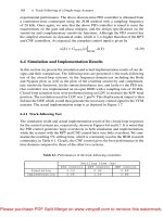
defines the family of parabolas. Let us define
to be the positioning
error with
being the desired final position. Then, if we consider the trajectories
between
and , our desired final state in and plane must be
(4.25)
In this case, the constants in the above trajectories are equal to zero. Moreover, both
of the trajectories given by Equations 4.23 and 4.24 are the decelerating trajectories
depending upon the direction of the travel. The mechanism of the TOC can be illus-
trated in a graphical form as given in Figure 4.1. Clearly, any initial state lying below
the curve is to be driven by the positive accelerating force to bring the state to the
Please purchase PDF Split-Merge on www.verypdf.com to remove this watermark.
100 4 Classical Nonlinear Control
−50
−40
−30
−20
−10
0
10
20
30
40
50
−150
−100
−50
0
50

100
150
e(t)
v(t)
P1
P2
u=−u
max
u=+u
max
u=+u
max
u=−u
max
Figure 4.1. Deceleration trajectories for TOC
deceleration trajectory. On the other hand, any initial state lying above the curve is
to be accelerated by the negative force to the deceleration trajectory.
Let
sgn (4.26)
The control law is then given by
sgn (4.27)
Figure 4.2. Typical scheme of TOC
A block diagram depicting the closed-loop method of bang-bang control is shown
in Figure 4.2. Unfortunately, the control law given by Equation 4.27 for the system
Please purchase PDF Split-Merge on www.verypdf.com to remove this watermark.
4.3 Proximate Time-optimal Servomechanism 101
shown in Figure 4.2, although time-optimal, is not practical. It applies maximum or
minimum input to the plant to be controlled even for a small error. Moreover, this
algorithm is not suited for disk drive applications for the following reasons:
1. even the smallest system process or measurement noise will cause control “chat-

ter”. This will excite the high-frequency modes.
2. any error in the plant model, will cause limit cycles to occur.
As such, the TOC given above has to be modified to suit HDD applications. In the
following section, we recall a modified version of the TOC proposed by Workman
[30], i.e. the PTOS. Such a control scheme is widely used nowadays in designing
HDD servo systems.
4.3 Proximate Time-optimal Servomechanism
The infinite gain of the signum function in the TOC causes control chatter, as seen in
the previous section. Workman [30], in 1987, proposed a modification of this tech-
nique, i.e. the so-called PTOS, to overcome such a drawback. The PTOS essentially
uses maximum acceleration where it is practical to do so. When the error is small,
it switches to a linear control law. To do so, it replaces the signum function in TOC
law by a saturation function. In the following sections, we revisit the PTOS method
in continuous-time and in discrete-time domains.
4.3.1 Continuous-time Systems
The configuration of the PTOS is shown in Figure 4.3. The function
is a finite-
slope approximation to the switching function
given by Equation 4.26. The
PTOS control law for the system in Equation 4.5 is given by
sat (4.28)
where sat
is defined as
Figure 4.3. Continuous-time PTOS
Please purchase PDF Split-Merge on www.verypdf.com to remove this watermark.
102 4 Classical Nonlinear Control
sat
if
if
if

(4.29)
and the function
is given by
for
sgn for
(4.30)
Here we note that
and are, respectively, the feedback gains for position and
velocity,
is a constant between and and is referred to as the acceleration dis-
count factor, and
is the size of the linear region. Since the linear portion of the
curve
must connect the two disjoint halves of the nonlinear portion, we have
constraints on the feedback gains and the linear region to guarantee the continuity of
the function
. It was proved by Workman [30] that
(4.31)
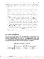
The control zones in the PTOS are shown in Figure 4.4. The two curves bounding
the switching curve (central curve) now redefine the control boundaries and it is
termed a linear boundary. Let this region be
. The region below the lower curve is
−400
−300
−200
−100
0
100
200
300

400
−400
−300
−200
−100
0
100
200
300
400
e(t)
v(t)
+u
max
−u
max
U
L
Figure 4.4. Control zones of a PTOS
Please purchase PDF Split-Merge on www.verypdf.com to remove this watermark.
4.3 Proximate Time-optimal Servomechanism 103
the region where the control , whereas the region above the upper curve
is the region where the control
. It has been proved [30] that once the
state trajectory enters the band
in Figure 4.4 it remains within and the control
signal is below the saturation. The region marked
is the region where the linear
control is applied.
The presence of the acceleration discount factor

allows us to accommodate
uncertainties in the plant accelerating factor at the cost of increase in response time.
By approximating the positioning time as the time that it takes the positioning error
to be within the linear region, one can show that the percentage increase
in time
taken by the PTOS over the time taken by the TOC is given by (see [30]):
(4.32)
Clearly, larger values of
make the response closer to that of the TOC. As a result
of changing the nonlinearity from sgn(
) to sat( ), the control chatter is eliminated.
4.3.2 Discrete-time Systems
The discrete-time PTOS can be derived from its continuous-time counterpart, but
with some conditions on sample time to ensure stability. In his seminal work,
Workman [30] extended the continuous-time PTOS to discrete-time control of a
continuous-time double-integrator plant driven by a zero-order hold as shown in
Figure 4.5. As in the continuous-time case, the states are defined as position and
velocity. With insignificant calculation delay, the state-space description of the plant
given by Equation 4.5 in the discrete-time domain is
(4.33)
where
is the sampling period. The control structure is a discrete-time mapping
of the continuous-time PTOS law, but with a constraint on the sampling period to
D/A
A/D
A/D
Discrete-
time
control
law

Figure 4.5. Discrete-time PTOS
Please purchase PDF Split-Merge on www.verypdf.com to remove this watermark.
104 4 Classical Nonlinear Control
guarantee that the control does not saturate during the deceleration phase to the target
position and also to guarantee its stability. Thus, the mapped control law is
sat (4.34)
with the following constraint on sampling frequency
,
(4.35)
where
is the desired bandwidth of the closed-loop system.
4.4 Mode-switching Control
In this section, we present a mode-switching control (MSC) design technique for
both continuous-time and discrete-time systems, which is a combination of the PTOS
of the previous section and the RPT technique given in Chapter 4.
4.4.1 Continuous-time Systems
In this subsection, we follow the development of [125] to introduce the design of an
MSC design for a system characterized by a double integrator or in the following
state-space equation:
(4.36)
where as usual
is the state, which consists of the displacement and the velocity
; is the control input constrained by
(4.37)
As will be seen shortly in the forthcoming chapters, the VCM actuators of HDDs
can generally be approximated by such a model with appropriate parameters
and
. In HDD servo systems, in order to achieve both high-speed track seeking and
highly accurate head positioning, multimode control designs are widely used. The
two commonly used multimode control designs are MSC and sliding mode control.

Both control techniques in fact belong to the category of variable-structure control.
That is, the control is switched between two or more different controllers to achieve
the two conflicting requirements. In this section, we propose an MSC scheme in
which the seeking mode is controlled by a PTOS and the track-following mode is
controlled by a RPT controller.
As noted earlier, the MSC (see, e.g., [15]) is a type of variable structure control
systems [126], but the switching is in only one direction. Figure 4.6 shows a basic
schematic diagram of MSC. There are track seeking and track following modes.
Please purchase PDF Split-Merge on www.verypdf.com to remove this watermark.