Tài liệu Hard Disk Drive Servo Systems- P6 pdf

8.4 Simulation and Implementation Results 239
which is the same as those in the previous chapters, to our servo systems. The im-
plementation results of the corresponding responses are respectively shown in Fig-
ures 8.20 to 8.22.
0
10
20
30
40
50
60
70
80
90
100
0.3
0.4
0.5
0.6
0.7
RRO disturbance (μm)
0
10
20
30
40
50
60
70
80
90

100
−0.05
0
0.05
Error (μm)
0
10
20
30
40
50
60
70
80
90
100
−0.05
0
0.05
Error (μm)
Time (ms)
Single−stage
Dual−stage
Figure 8.20. Implementation results: Responses to a runout disturbance (PID)
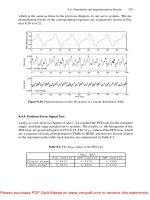
8.4.4 Position Error Signal Test
Lastly, as were done in Chapters 6 and 7, we conduct the PES tests for the complete
single- and dual-stage actuated servo systems. The results, i.e. the histograms of the
PES tests, are given in Figures 8.23 to 8.25. The 3
values of the PES tests, which
are a measure of track misregistration (TMR) in HDDs and that are closely related

to the maximum achievable track density, are summarized in Table 8.2.
Table 8.2. The values of the PES tests
3 (
l
um)
PID control RPT control CNF control
Single-stage 0.0615 0.0375 0.0288
Dual-stage 0.0273 0.0204 0.0195
Please purchase PDF Split-Merge on www.verypdf.com to remove this watermark.
240 8 Dual-stage Actuated Servo Systems
0
10
20
30
40
50
60
70
80
90
100
0.3
0.4
0.5
0.6
0.7
RRO disturbance (μm)
0
10
20

30
40
50
60
70
80
90
100
−0.05
0
0.05
Error (μm)
0
10
20
30
40
50
60
70
80
90
100
−0.05
0
0.05
Error (μm)
Time (ms)
Single−stage
Dual−stage

Figure 8.21. Implementation results: Responses to a runout disturbance (RPT)
0
10
20
30
40
50
60
70
80
90
100
0.3
0.4
0.5
0.6
0.7
RRO disturbance (μm)
0
10
20
30
40
50
60
70
80
90
100
−0.05

0
0.05
Error (μm)
0
10
20
30
40
50
60
70
80
90
100
−0.05
0
0.05
Error (μm)
Time (ms)
Single−stage
Dual−stage
Figure 8.22. Implementation results: Responses to a runout disturbance (CNF)
Please purchase PDF Split-Merge on www.verypdf.com to remove this watermark.
8.4 Simulation and Implementation Results 241
−0.1
−0.05
0
0.05
0.1
0

1000
2000
3000
4000
5000
6000
Error (μm)
Points
−0.1
−0.05
0
0.05
0.1
0
1000
2000
3000
4000
5000
6000
Error (μm)
Points
Single−stage
Dual−stage
Figure 8.23. Implementation results: PES test histograms (PID)
−0.1
−0.05
0
0.05
0.1

0
1000
2000
3000
4000
5000
6000
Error (μm)
Points
−0.1
−0.05
0
0.05
0.1
0
1000
2000
3000
4000
5000
6000
Error (μm)
Points
Single−stage Dual−stage
Figure 8.24. Implementation results: PES test histograms (RPT)
Please purchase PDF Split-Merge on www.verypdf.com to remove this watermark.
242 8 Dual-stage Actuated Servo Systems
−0.1
−0.05
0

0.05
0.1
0
1000
2000
3000
4000
5000
6000
Error (μm)
Points
−0.1
−0.05
0
0.05
0.1
0
1000
2000
3000
4000
5000
6000
Error (μm)
Points
Single−stage
Dual−stage
Figure 8.25. Implementation results: PES test histograms (CNF)
It can be easily observed from the results obtained that the dual-stage actuated
servo systems do provide a faster settling time and better positioning accuracy com-

pared with those of the single-stage actuated counterparts. The improvement in the
track-following stage turns out to be very noticeable. This was actually the origi-
nal purpose of introducing the microactuator into HDD servo systems. However, we
personally feel that the price we have paid (i.e. by adding an expensive and delicate
piezoelectric actuator to the system) for such an improvement is too high.
Please purchase PDF Split-Merge on www.verypdf.com to remove this watermark.
9
Modeling and Design of a Microdrive System
9.1 Introduction
Chapters 6 to 8 focus on the design of single- and dual-stage actuated hard drive servo
systems. The hard drives considered are those used in normal desktop computers.
As mentioned earlier in the introduction chapter, microdrives have become popular
these days because of high demand from many new applications. Many factors such
as frictional forces and nonlinearities, which are negligible for normal drives and
thus ignored in servo systems given in Chapters 6 to 8, emerge as critical issues for
microdrives. It can be observed that nonlinearities from friction in the actuator rotary
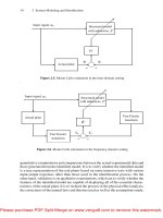
pivot bearing and data flex cable in the VCM actuator (see Figure 9.1) generate large
residual errors and deteriorate the performance of head positioning of HDD servo
systems, which is much more severe in the track-following stage when the R/W
head is moving from the current track to its neighborhood tracks. The desire to fully
understand the behaviors of nonlinearities and friction in microdrives is obvious.
Actually, this motivates us to carry out a complete study and modeling of friction
and nonlinearities for the VCM-actuated HDD servo systems.
Friction is hard nonlinear and may result in residual errors, limit cycles and poor
performance (see, e.g., [168–171]. Friction exists in almost all servomechanisms,
behaves in features of the Stribeck effect, hysteresis, stiction and varying break-away
force, occurs in all mechanical systems and appears at the physical interface between
two contact surfaces moving relative to each other. The features of friction have been
extensively studied (see, e.g., [168–174]), but there are significant differences among
diverse systems. There has been a significantly increased interest in friction in the

industry, which is driven by strong engineering needs in a wide range of industries
and availability of both precise measurement and advanced control techniques.
The HDD industry persists in the need for companies to come up with devices
that are cheaper and able to store more data and retrieve or write to them at faster
speed. Decreasing the HDD track width is a feasible idea to achieve these objectives.
But, the presence of friction in the rotary actuator pivot bearing results in large resid-
ual errors and high-frequency oscillations, which may produce a larger positioning
error signal to hold back the further decreasing of the track width and to degrade
Please purchase PDF Split-Merge on www.verypdf.com to remove this watermark.
244 9 Modeling and Design of a Microdrive System
Figure 9.1. An HDD with a VCM actuator
the performance of the servo systems. This issue becomes more noticeable for small
drives and is one of the challenges to design head positioning servo systems for small
HDDs. Much effort has been put into the research on mitigation of the friction in the
pivot bearing in the HDD industry in the last decade (see, e.g., [8, 175–178]). It is
still ongoing in the disk drive industry (see, e.g., [69, 179, 180]).
Diverse modeling methods had been proposed (see, e.g., [59, 69]) based on linear
systems, where nonlinearities of plants are assumed to be tiny and can be neglected.
As such, these methods cannot be directly applied to model plants with significant
nonlinearities. Instead, in the first part of this chapter, we utilize the physical ef-
fect approach given in Chapter 2 to determine the structures of nonlinearities and
friction associated with the VCM actuator in a typical HDD servo system. This is
done by carefully examining and analyzing physical effects that occur in or between
electromechanical parts. Then, we employ a Monte Carlo process (see Chapter 2) to
identify the parameters in the structured model. We note that Monte Carlo methods
are very effective in approximating solutions to a variety of mathematical problems,
for which their analytical solutions are hard, if not impossible, to determine. Our
simulation and experimental results show that the identified model of friction and
nonlinearities using such approaches matches very well the behavior of the actual
system.

The second part of this chapter focuses on the controller design for the HDD
servo system. Our philosophy of designing servo systems is rather simple. Once the
model of the friction and nonlinearities of the VCM actuator is obtained, we will try
to cancel as much as possible all these unwanted elements in the servo system. As it
is impossible to have perfect models for friction and nonlinearities, a perfect cancel-
lation of these elements is unlikely to happen in the real world. We then formulate
our design by treating the uncompensated portion as external disturbances. The PID
Please purchase PDF Split-Merge on www.verypdf.com to remove this watermark.
9.2 Modeling of the Microdrive Actuator 245
and RPT control techniques of Chapter 3 and the CNF control technique of Chapter 5
are to be used to carry out our servo system design. We note that some of the results
presented in this chapter have been reported earlier in [138].
9.2 Modeling of the Microdrive Actuator
The physical structure of a typical VCM actuator is shown in Figure 9.2. The motion
of the coil is driven by a permanent magnet similar to typical DC motors. The stator
of the VCM is built of a permanent magnet. The rotor consists of a coil, a pivot
and a metal arm on which the R/W head is attached. A data flex cable is connected
with the R/W head through the metal arm to transfer data read from or written to
the HDD disc via the R/W head. Typically, the rotor has a deflected angle,
in rad,
ranging up to
rad in commercial disk drives. We are particularly interested in
the modeling of the friction and nonlinearities for the actuator in the track-following
stage, in which the R/W head movement is within the neighborhood of its current
track and thus
. An IBM microdrive (DMDM-10340) is used throughout for
illustration.
SN
I
Magnet

Permanent
Coil
Pivot
R/W Head
α
Figure 9.2. The mechanical structure of a typical VCM actuator
9.2.1 Structural Model of the VCM Actuator
We first adopt the physical effect analysis of Chapter 2 to determine the structures of
nonlinearities in the VCM actuator. It is to analyze the effects between the compo-
nents of the actuator, such as the stator, rotor and support plane as well as the VCM
driver. The VCM actuator is designed to position the R/W head fast and precisely
Please purchase PDF Split-Merge on www.verypdf.com to remove this watermark.
246 9 Modeling and Design of a Microdrive System
onto the target track, and is driven by a VCM driver, a full bridge power amplifier,
which converts an input voltage into an electric current. The electrical circuit of a
typical VCM driver is shown in Figure 9.3, where
represents the coil of the VCM
actuator and the external input voltage is exerted directly into the VCM driver to
drive the coil.
In order to simplify our analysis, we assume that the physical system has the fol-
lowing properties: i) the permanent magnet is constant; and ii) the coil is assembled
strictly along the radius and concentric circle of the pivot; Furthermore, we assume
that the friction of a mechanical object consists of Coloumb friction and viscous
damping, and is characterized by a typical friction function as follows:
N
N
sgn
N
N
sgn

N
(9.1)
where
is the friction force,
N
is the normal force, i.e. the force perpendicular to the
contacted surfaces of the objects,
is the external force applied to the object, is
the relative moving speed between two contact surfaces, and
N
is the breakaway
force. Furthermore,
, and are, respectively, the dynamic, static and viscous
coefficients of friction.
Through a detailed analysis of the VCM driver circuit in Figure 9.3, it is straight-
forward to verify that the relationship between the driver input voltage and the current
and voltage of the VCM coil is given by
(9.2)
where
(9.3)
A
B
C
Figure 9.3. The electrical circuit of a typical VCM driver
Please purchase PDF Split-Merge on www.verypdf.com to remove this watermark.
9.2 Modeling of the Microdrive Actuator 247
is the input voltage to the VCM driver, and are, respectively, the VCM coil
current and voltage. For the IBM microdrive (DMDM-10340) used in our experi-
ment,
k , k , k , , k , pF,

and the amplifier gains
and . For such a drive, we have
(9.4)
which has a magnitude response ranging from
dB (for frequency less than 110
Hz) to
dB (for frequency greater than 2.2 kHz), and
for all (9.5)
Such a property generally holds for all commercial disk drives. As such, it is safe to
approximate the relationship of
and of the VCM driver as
(9.6)
For the IBM microdrive used in this work,
.
Next, it is straightforward to derive that the torque
, relative to the center of
the pivot and that moving anticlockwise is positive and produced by the permanent
magnet
in the coil with the electric current, is given by
(9.7)
and are, respectively, the outside and inside radius of the coil to the center of
the pivot, and
is the number of windings of the coil. The total external torque
applied to the VCM actuator is given as follows:
(9.8)
where
is the spring torque produced by the data flex cable and is a function
of the deflection angle
or the displacement of the R/W head. The friction torque
in the VCM actuator comes from two major sources: One is the friction in the pivot

bearing and the other is between the pivot bearing and the support plane. The friction
torque in the pivot bearing can be characterized as
N
(9.9)
where
is the external force, , and are the related friction coefficients
as defined in Equation 9.1,
is the radius of the pivot to its center, and
N
(9.10)
is the normal force, which consists of the centrifugal force of the rotor and the dia-
metrical force,
. Furthermore, is a constant dependent on the mass distribution
of the rotor, and
Please purchase PDF Split-Merge on www.verypdf.com to remove this watermark.
248 9 Modeling and Design of a Microdrive System
(9.11)
is the force along the radius of the pivot bearing produced in the coil by the permanent
magnet.
The friction torque between the pivot bearing and the support plane can be char-
acterized as:
N
(9.12)
where
is the external force, , and are the related friction coefficients
as defined in Equation 9.1, and
N
(9.13)
is the normal force resulted from a static balance torque of the rotor,
. Thus, the

total friction torque
presented in the VCM actuator is given by
and
sgn and
(9.14)
where
sgn
(9.15)
and
(9.16)
is the breakaway torque, and where
and are, respectively, the corresponding
input voltage and the deflection angle for the situation when
.
Lastly, it is simple to verify that the relative displacement of the R/W head,
,is
given by
sin (9.17)
where
is the length from the R/W head to the center of the pivot. Following New-
ton’s law of motion,
, where is the moment of inertia of the VCM
rotor, we have
(9.18)
where
sgn
sgn
(9.19)
where
Please purchase PDF Split-Merge on www.verypdf.com to remove this watermark.

9.2 Modeling of the Microdrive Actuator 249
(9.20)
with
and being, respectively, the corresponding input voltage and the displace-
ment for the case when
. It is clear now that the expressions in Equations
9.18–9.20 give a complete structure of the VCM model including friction and non-
linearities from the data flex cable. Our next task is to identify all these parameters
for the IBM microdrive (DMDM-10340).
9.2.2 Identification and Verification of Model Parameters
We proceed to identify the parameters of the VCM actuator model given in Equations
9.18–9.20. We note that there are results available in the literature (see, e.g., [168])
to estimate friction parameters for typical DC motors for which both velocity and
displacement are measurable and without constraint. Unfortunately, for the VCM
actuator studied in this chapter, it is impossible to measure the time responses in
constant-velocity motions and only the relative displacement of the R/W head is
measurable. As such, the method of [168] cannot be adopted to solve our problems.
Instead, we employ the popular Monte Carlo method of Chapter 2 (see also, [63–
65]), which has been widely used in solving engineering problems and is capable of
providing good numerical solutions.
First, it is simple to obtain from Equation 9.18 at a steady state when
and
,
(9.21)
Our experimental results show that the right hand side of Equation 9.21 is very in-
significant for small input signal
and small displacement . This will be verified
later when the model parameters are fully identified. Thus, we have
(9.22)
which is used to identify

or equivalently , the spring torque produced by
the data flex cable. Next, for the small neighborhood of
, we can rewrite the
dynamic expression of Equation 9.18 as
(9.23)
Please purchase PDF Split-Merge on www.verypdf.com to remove this watermark.
250 9 Modeling and Design of a Microdrive System
For small signals, and by omitting the nonlinear terms in , the system dynamics in
Equation 9.23 can be approximated by a second-order linear system with a transfer
function from
to :
(9.24)
The natural frequency of the above transfer function (or roughly its peak frequency),
, is given by
(9.25)
and its static gain is given by
, which implies that
(9.26)
where
. The expression in Equation 9.26 will be used to estimate the
parameter
. More specifically, the parameters of the dynamic models of the VCM
actuator will be identified using the following procedure:
1. The nonlinear characteristics of the data flex cable or equivalently
will
be initially determined using Equation 9.22 with a set of input signal,
, and
its corresponding output displacement,
. It will be fine tuned later using the
Monte Carlo method.

2. The parameter
will be initially computed using measured static gains and peak
frequencies as in Equation 9.26, resulting from the dynamical responses of the
actuator to a set of small input signals. Again, the identified parameter will be
fine tuned later using the Monte Carlo method.
3. All system parameters will then be identified using the Monte Carlo method to
match the frequency response to small input signal;
4. The high-frequency resonance modes of the actuator, which have not been in-
cluded in either Equation 9.18 or 9.23, will be determined from frequency re-
sponses to input signals at high frequencies.
The above procedure will yield a complete and comprehensive model including nom-
inal dynamics, high-frequency resonance modes, friction and nonlinearities of the
VCM actuator. In our experiments, the relative displacement of the R/W head is the
only measurable output and is measured using a laser Doppler vibrometer (LDV). A
dynamic signal analyzer (DSA) (Model SRS 785) is used to measure the frequency
responses of the VCM actuator. The DSA is also used to record both input and output
signals of time-domain responses. Square waves are generated with a dSpace DSP
board installed in a personal computer.
The time-domain response of the VCM actuator to a typical square input signal
about
Hz is shown in Figure 9.4. With a group of time-domain responses to a
set of square input signals, we obtain the corresponding measurement data for the
nonlinear function,
, which can be matched nicely by an arctan function (see
Figure 9.5) as follows:
Please purchase PDF Split-Merge on www.verypdf.com to remove this watermark.
9.2 Modeling of the Microdrive Actuator 251
0
0.1
0.2

0.3
0.4
0.5
0.6
0.7
0.8
−0.005
0
0.005
0.01
0.015
0.02
0.025
Time (s)
Input signal to VCM (V)
0
0.1
0.2
0.3
0.4
0.5
0.6
0.7
0.8
−0.5
0
0.5
1
1.5
2

2.5
3
3.5
Time (s)
Displacement (μm)
Solid line: experimental
Dashed line: average
Figure 9.4. Time-domain response of the VCM actuator to a square wave input
−10
−8
−6
−4
−2
0
2
4
6
8
−0.03
−0.02
−0.01
0
0.01
0.02
0.03
Displacement (μm)
Functional value (V)
Solid line: Experimental data
Dashed line: Identified function
Figure 9.5. Nonlinear characteristics of the data flex cable

Please purchase PDF Split-Merge on www.verypdf.com to remove this watermark.
252 9 Modeling and Design of a Microdrive System
(9.27)
where
V and (
l
um) . These parameters will be
further fine tuned later in the Monte Carlo process.
Next, by fixing a particular input offset point
and by injecting on top of a
sweep of small sinusoidal signals with an amplitude of
mV, we are able to obtain a
corresponding frequency response within the range of interest. It then follows from
Equation 9.26 that the values of the static gain,
, and peak frequency, ,ofthe
frequency response can be used to estimate the parameter,
. Figure 9.6 shows the
frequency response of the system for the pair
, which gives a static
gain of
and a peak frequency of Hz. In order to obtain a more accurate
result, we repeat the above experimental tests for several pairs
and the results
are shown in Table 9.1. The parameter,
, can then be more accurately determined
from these data using a least square fitting,
(9.28)
which gives an optimal solution
l
um / (Vs

). Nonetheless, this param-
eter will again be fine tuned later in the Monte Carlo process.
Lastly, we apply a Monte Carlo process to identify all other parameters of our
VCM actuator model and to fine tune those parameters, which have previously
been identified. Monte Carlo processes are known as numerical simulation methods
10
0
10
1
10
2
0
10
20
30
40
50
Frequency (Hz)
Magnitude (dB)
Solid line: experimental
Dashed line: identified
10
0
10
1
10
2
−250
−200
−150

−100
−50
0
50
Frequency (Hz)
Phase (deg)
Figure 9.6. Frequency response to small signals at the steady state with
Please purchase PDF Split-Merge on www.verypdf.com to remove this watermark.
9.2 Modeling of the Microdrive Actuator 253
Table 9.1. Static gains and peak frequencies of the actuator for small inputs
(mV)
60.73 59.06 63.71 62.43 63.72 65.12 65.50
(Hz) 310.30 310.63 305.24 303.88 299.56 296.99 295.43
that make use of random numbers and probability statistics to solve some compli-
cated mathematical problems. The detailed treatments of Monte Carlo methods vary
widely from field to field. Originally, a Monte Carlo experiment means to use ran-
dom numbers to examine some stochastic problems. The idea can be extended to
deterministic problems by presetting some parameters and conditions of the prob-
lems. The use of Monte Carlo methods for modeling physical systems allows us to
solve more complicated problems, and provides approximate solutions to a variety
of mathematical problems, whose analytical solutions are hard, if not impossible,
to derive. In what follows, a Monte Carlo process is utilized to obtain time-domain
responses of the VCM actuator model in Equation 9.18 with a set of preset param-
eters
and input signals. The corresponding frequency
responses are obtained through Fourier transformation of the obtained time-domain
responses. Our idea of using the Monte Carlo process is to minimize the differences
between simulated frequency responses and the experimental ones by iteratively ad-
justing the parameters of the physical model in Equation 9.18. The input signals in
our simulations are again a combination of an offset

and sinusoidal signals with
a small amplitude
mV and several frequencies ranging from 1 Hz to 1 kHz.
Although Monte Carlo methods can only give locally minimal solutions, in our
problem, however, the predetermined nonlinear characteristics of the data flex cable
and the parameter,
, have given us a rough idea on what the true solution should
be. The solution within the neighborhood of the previously identified parameters are
given by
l
um / (V
s )
V
(
l
um)
s
(
l
um)
(
l
um)
l
um / s
(
l
um)
l
um / s

(9.29)
These parameters will be used for further verifications using the experimental setup
of the actual system.
So far, we have only focused on the low-frequency components of the VCM ac-
tuator model. In fact, there are many high-frequency resonance modes, which are
Please purchase PDF Split-Merge on www.verypdf.com to remove this watermark.
254 9 Modeling and Design of a Microdrive System
crucial to the overall performance of HDD servo systems. The high-frequency res-
onance modes of the VCM actuator can be obtained from frequency responses of
the system in the high-frequency region (see Figure 9.7). The transfer function that
matches the frequency responses given in Figure 9.7 is identified using the standard
least square estimation method of Chapter 2 and is characterized by
(9.30)
with the resonance modes being given as
(9.31)
(9.32)
(9.33)
(9.34)
and
(9.35)
Finally, for easy reference, we conclude this section by explicitly expressing the
identified rigid model of VCM actuator:
(9.36)
where
sgn
sgn
(9.37)
and where
(9.38)
(9.39)

with
and being, respectively, the corresponding input voltage and the displace-
ment for the case when
. Note that in the above model, the input signal
is in voltage and the output displacement is in micrometers. Together with the
high-frequency resonance modes of Equations 9.31–9.35, the above model presents
a comprehensive characterization of the VCM actuator studied. This model will be
further verified using experimental tests on the actual system.
Please purchase PDF Split-Merge on www.verypdf.com to remove this watermark.
9.3 Microdrive Servo System Design 255
10
3
10
4
−60
−40
−20
0
20
40
Magnitude (dB)
Frequency (Hz)
Solid line: experimental
Dashed line: identified
10
3
10
4
−900
−800

−700
−600
−500
−400
−300
−200
Phase (Deg)
Frequency (Hz)
Figure 9.7. Frequency responses of the VCM actuator in the high-frequency region
In order to verify the validity of the established model of the VCM actuator, we
carry out a series of comparisons between the experimental results and computed
results of the time-domain responses and frequency-domain responses of the actu-
ator. The comparison of the frequency responses between the experimental result
and the identified result for inputs consisting of
mV and sine waves with
amplitude of 1 mV is shown in Figure 9.8. It clearly shows that the result of the
identified model matches well with the experimental result. The comparison of the
time-domain responses for an input signal consisting of
mV and a sine
wave with an amplitude of 5 mV is given in Figure 9.9. It shows that the simula-
tion results match the trends and values of those obtained from experiments. The
noises associated with experimental results in Figures 9.8 and 9.9 are drift noises
caused by the LDV and/or DSA. The comparisons of both frequency-domain and
time-domain responses demonstrate that the identified model of the VCM actuator
indeed describes the features of the actuator.
9.3 Microdrive Servo System Design
We proceed to design a servo system for the microdrive identified in Section 9.2.
As mentioned earlier, our design philosophy is rather simple. We make full use of
the obtained model of the friction and nonlinearities of the VCM actuator to design
a precompensator, which would cancel as much as possible all the unwanted ele-

ments in the servo system. As it is impossible to have perfect models for friction
Please purchase PDF Split-Merge on www.verypdf.com to remove this watermark.
256 9 Modeling and Design of a Microdrive System
10
0
10
1
10
2
0
10
20
30
40
50
Frequency (Hz)
Magnitude (dB)
Solid line: experimental
Dashed line: identified
10
0
10
1
10
2
−250
−200
−150
−100
−50

0
50
Frequency (Hz)
Phase (deg)
Figure 9.8. Comparison of frequency responses to small signals of actuator with mV
0
0.2
0.4
0.6
0.8
1
1.2
1.4
1.6
1.8
2
−10
−8
−6
−4
−2
0
x 10
−3
Time (s)
Input signal to VCM (V)
0
0.2
0.4
0.6

0.8
1
1.2
1.4
1.6
1.8
2
−1
−0.8
−0.6
−0.4
−0.2
0
0.2
Time (s)
Displacement (μm)
Solid line: experimental
Dashed line: simulated
Figure 9.9. Comparison of time-domain responses of the VCM actuator
Please purchase PDF Split-Merge on www.verypdf.com to remove this watermark.
9.3 Microdrive Servo System Design 257
HDD
Nonlinearity
compensation
Enhanced
CNF controller
Figure 9.10. Control scheme for the HDD servo system
and nonlinearities, a perfect cancellation of these elements is unlikely to happen in
the real world. We then formulate our design by treating the uncompensated portion
as external disturbances. The enhanced CNF control technique of Chapter 5 is then

employed to design an effective tracking controller. The overall control scheme for
the servo system is depicted in Figure 9.10. Although we focus our attention here
on HDD, it is our belief that such an approach can be adopted to solve other servo
problems.
Examining the model of Equation 9.36, it is easy to obtain a precompensation,
(9.40)
which would eliminate the majority of nonlinearities in the data flex cable. The HDD
model of Equation 9.18 can then be simplified as follows:
sat
(9.41)
where the disturbance,
, represents uncompensated nonlinearities, and is the
relative displacement of the R/W head (in micrometers). The control input,
,isto
be limited within
with V.
We design a microdrive servo system that meets the following design constraints
and specifications:
1. the control input does not exceed
V owing to physical constraints on the
actual VCM actuator;
2. the overshoot and undershoot of the step response are kept to less than 5% as the
R/W head can start to read or write within
of the target;
Please purchase PDF Split-Merge on www.verypdf.com to remove this watermark.
258 9 Modeling and Design of a Microdrive System
3. the 5% settling time in the step response is as short as possible;
4. the gain margin and phase margin of the overall design are, respectively, greater
than 6 dB and
;

5. the maximum peaks of the sensitivity and complementary sensitivity functions
are less than 6 dB; and
6. the sampling frequency in implementing the actual controller is 20 kHz.
It turns out that for the microdrive its resonance modes are at very high frequen-
cies that are far above the working range of the drive. It is thus not necessary to add
a notch filter to minimize their effects. As usual, we consider a second-order nom-
inal model of Equation 9.41 for the VCM actuator. The resonance modes and the
notch filter will be put back to evaluate the performance of the overall design. As
in Chapters 6 and 8, we design our servo system using, respectively, PID, RPT and
CNF control.
1. The PID control law (discretized with a sampling frequency of 20 kHz) is given
by
(9.42)
2. The RPT controller is given by
(9.43)
and
(9.44)
3. Finally, the CNF control law is given as follows:
sat
(9.45)
and
(9.46)
where
(9.47)
Please purchase PDF Split-Merge on www.verypdf.com to remove this watermark.