Tài liệu GPS - đường dẫn quán tính và hội nhập P8 doc

8
Kalman Filter Engineering
We now consider the following, practical aspects of Kalman ®ltering applications:
1. how performance of the Kalman ®lter can degrade due to computer roundoff
errors and alternative implementation methods with better robustness against
roundoff;
2. how to determine computer memory, word length, and throughput require-
ments for implementing Kalman ®lters in computers;
3. ways to implement real-time monitoring and analysis of ®lter performance;
4. the Schmidt±Kalman suboptimal ®lter, designed for reducing computer
requirements;
5. covariance analysis, which uses the Riccati equations for performance-based
predictive design of sensor systems; and
6. Kalman ®lter architectures for GPS/INS integration.
8.1 MORE STABLE IMPLEMENTATION METHODS
8.1.1 Effects of Computer Roundoff
Computer roundoff limits the precision of numerical representation in the imple-
mentation of Kalman ®lters. It has been shown to cause severe degradation of ®lter
performance in many applications, and alternative implementations of the Kalman
®lter equations (the Riccati equations, in particular) have been shown to improve
robustness against roundoff errors.
229
Global Positioning Systems, Inertial Navigation, and Integration,
Mohinder S. Grewal, Lawrence R. Weill, Angus P. Andrews
Copyright # 2001 John Wiley & Sons, Inc.
Print ISBN 0-471-35032-X Electronic ISBN 0-471-20071-9
Computer roundoff for ¯oating-point arithmetic is often characterized by a single
parameter e
roundoff
, which is the largest number such that
1  e

roundoff
 1 in machine precision. 8:1
The following example, due to Dyer and McReynolds [32], shows how a problem
that is well conditioned, as posed, can be made ill-conditioned by the ®lter
implementation.
Example 8.1 Let I
n
denote the n  n identity matrix. Consider the ®ltering problem
with measurement sensitivity matrix
H 
11 1
111 d
!
and covariance matrices
P
0
 I
3
,andR  d
2
I
2
;
where d
2
< e
roundoff
but d > e
roundoff
. In this case, although H clearly has rank 2 in

machine precision, the product HP
0
H
T
with roundoff will equal
33 d
3  d 3 2d
!
;
which is singular. The result is unchanged when R is added to HP
0
H
T
. In this case,
then, the ®lter observational update fails because the matrix HP
0
H
T
 R is not
invertible.
8.1.2 Alternative Implementations
The covariance correction process (observational update) in the solution of the
Riccati equation was found to be the dominant source of numerical instability in the
Kalman ®lter implementation, with the more common symptoms of failure being
asymmetry of the covariance matrix (easily ®xed) or, worse by far, negative terms on
its diagonal. These implementation problems could be avoided for some problems
by using more precision, but they were eventually solved for most applications by
using alternatives to the covariance matrix P as the dependent variable in the
covariance correction equation. However, each of these methods required a com-
patible method for covariance prediction. Table 8.1 lists several of these compatible

implementation methods for improving the numerical stability of Kalman ®lters.
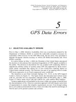
Figure 8.1 illustrates how these methods perform on the ill-conditioned problem
of Example 8.1 as the conditioning parameter d  0. For this particular test case,
using 64-bit ¯oating-point precision (52-bit mantissa), the accuracy of the Carlson
230
KALMAN FILTER ENGINEERING
TABLE 8.1 Compatible Methods for Implementing the
Riccati Equation
Covariance Implementation Methods
Matrix Corrector Predictor
Format Method Method
Symmetric
nonnegative
de®nite
Kalman [71],
Joseph [19]
Kalman [71]
Kalman [71]
Square
Cholesky
factor C
Potter
[100, 8]
C
k1
  F
k
C
k


Triangular
Cholesky
factor C
Carlson [20] Kailath±Schmidt
a
Triangular
Cholesky
factor C
Morf±Kailath combined [93]
Modi®ed
Cholesky
factors U; D
Bierman [10] Thornton [116]
a
From unpublished sources.
Fig. 8.1 Degradation of numerical solutions with problem conditioning.
8.1 MORE STABLE IMPLEMENTATION METHODS
231
[20] and Bierman [10] implementations degrade more gracefully than the others as
d  e, the machine precision limit. The Carlson and Bierman solutions still
maintain about nine digits (30 bits) of accuracy at d 

e

, when the other
methods have essentially no bits of accuracy in the computed solution.
These results, by themselves, do not prove the general superiority of the Carlson
and Bierman solutions for the Riccati equation. Relative performance of alternative
implementation methods may depend upon details of the speci®c application, and
for many applications, the standard Kalman ®lter implementation will suf®ce. For

many other applications, it has been found suf®cient to constrain the covariance
matrix to remain symmetric.
8.1.3 SerialMeasurement Processing
It is shown in [73] that it is more ef®cient to process the components of a
measurement vector serially, one component at a time, than to process them as a
vector. This may seem counterintuitive, but it is true even if its implementation
requires a transformation of measurement variables to make the associated measure-
ment noise covariance R a diagonal matrix (i.e., with noise uncorrelated from one
component to another).
8.1.3.1 Measurement Decorrelation If the covariance matrix R of measure-
ment noise is not a diagonal matrix, then it can be made so by UDU
T
decomposition
(Eq. B.22) and changing the measurement variables,
R
corr
 U
R
D
R
U
T
R
; 8:2
R
decorr

def
D
R

(a diagonal matrix); 8:3
z
decorr

def
U
R
z
corr
; 8:4
H
decorr

def
U
R
H
corr
; 8:5
where R
corr
is the nondiagonal (i.e., correlated component to component) measure-
ment noise covariance matrix, and the new decorrelated measurement vector z
decorr
has a diagonal measurement noise covariance matrix R
decorr
and measurement
sensitivity matrix H
decorr
.

8.1.3.2 Serial Processing of Decorrelated Measurements The compo-
nents of z
decorr
can now be processed one component at a time using the
corresponding row of H
decorr
as its measurement sensitivity matrix and the
corresponding diagonal element of R
decorr
as its measurement noise variance.
A MATLAB implementation for this procedure is listed in Table 8.2, where the
®nal line is a ``symmetrizing'' procedure designed to improve robustness.
232
KALMAN FILTER ENGINEERING
8.1.4 Joseph Stabilized Implementation
This implementation of the Kalman ®lter is in [19], where it is demonstrated that
numerical stability of the solution to the Riccati equation can be improved by
rearranging the standard formulas for the measurement update into the following
formats (given here for scalar measurements):
z 
z

R

; 8:6

H  zH; 8:7
K 

HP


H
T
 1
1
P

H
T
; 8:8
P I 
K

HPI  K

H
T
 K K
T
: 8:9
These equations would replace those for
K and P within the loop in Table 8.2.
The Joseph stabilized implementation and re®nements (mostly taking advantage
of partial results and the redundancy due to symmetry) in [10], [46] and are
implemented in the MATLAB ®les Joseph.m, Josephb.m,andJosephdv.m,
respectively, on the accompanying diskette.
8.1.5 Factorization Methods
8.1.5.1 Historical Background Robust implementation methods were intro-
duced ®rst for the covariance correction (measurement updates), observed to be the
principal source of numerical instability. In [100, 8], the idea of using a Cholesky

factor (de®ned in Section B.8.1) of the covariance matrix P, as the dependent
variable in the Riccati equation is introduced.
Carlson [20] discovered a more robust method using triangular Cholesky factors,
which have zeros either above or below their main diagonals. Bierman [10] extended
TABLE 8.2 Matlab Implementation of
SerialMeasurement Update
x = x
Ã
k
[-]
P = P
k
[-]
for j=1: `,
z=z
k
(j),
H = H
k
(j,:);
R
= R
decorr
(j,j);
K=
PH'/(HPH'+R)
x =
K(
z
-Hx);

P =
P-KHP;
end;
x
Ã
k
[+]
= x
P
k
[+]
=(P+
P')/2;
8.1 MORE STABLE IMPLEMENTATION METHODS
233
this to modi®ed Cholesky factors (de®ned in Section B.1.8.1), which are diagonal
and unit triangular matrices D and U, respectively, such that
UDU
T
 P 8:10
and U is triangular with 1's along its main diagonal.
Compatible covariance prediction methods were discovered by Thomas Kailath
and Stanley F. Schmidt (for Carlson's method) and Catherine Thornton [116] (for
Bierman's method).
8.1.6 Square-Root Filtering Methods
8.1.6.1 Problems with the Riccati Equation Many early applications of
Kalman ®ltering ran into serious numerical instability problems in solving the
ancillary Riccati equation for the Kalman gain. The problem was eventually solved
(over the next decade or so) by reformulating the Riccati equation so that its solution
was more robust against computer roundoff errors. Some of the more successful of

these approaches are collectively called ``square-root ®ltering.''
8.1.6.2 Square-Root Filtering The concept for square-root ®ltering came
from James H. Potter when he was at the MIT Instrumentation Laboratory (later the
Charles Stark Draper Laboratory) in the early 1960s, and his concept was
implemented successfully in the Kalman ®lter used for onboard navigation in all
the Apollo moon missions. Potter's algorithm is implemented on the Matlab m-®le
potter.m on the accompanying diskette. It was originally called square-root
®ltering because it is based, in part, on an algorithm for taking a symmmetric square
root of a special form of a symmetric matrix.
The improved robustness of Potter's approach comes from replacing the covar-
iance matrix P with its Cholesky factor
1
as the dependent parameter of the Riccati
equation. Some of the observed improvement in numerical stability is attributed to
improvement in the condition number condC (ratio of largest to smallest char-
acteristic value) over condP, because
condC

condP
p
: 8:11
A matrix is considered ill-conditioned for inversion in a particular computer
(``machine'' ) if its condition number is close to 1=e
machine
, where e
machine
is the
largest positive number
2
for which

1  e
machine

machine
1 8:12
1
See Section B.1.8.1 for the de®nition and properties of Cholesky factors.
2
e
machine
has the reserved name eps in MATLAB. Its value is returned when you type ``eps''.
234
KALMAN FILTER ENGINEERING
in machine precision. That is, the result of adding e
machine
to 1 has no effect in
machine precision.
8.1.6.3 Triangularization Methods The so-called ``QR'' theorem of linear
algebra states that every real m  n matrix S can be factored in the form S  QR,
where Q is an m  m orthogonal matrix and R is an m  n upper triangular matrix.
Depending on the relative magnitudes of m and n, the resulting triangular matrix R
may have any of the forms
m < nm nm< n
R 
with the nonzero part of the upper triangular submatrix in the upper right corner.
There are several algorithms for computing the triangular and orthogonal factors,
including some with the order of the factors reversed (effectively ``RQ'' algorithms).
These are also called triangularization methods. They are key to square-root
®ltering, because they can transform a nontriangular Cholesky factor M into a
triangular one


T, because
MM
T


T

O

O
T

T
T
8:13


T

T
T
: 8:14
Algorithms that implement QR decompositions need not compute the orthogonal
factor explicitly, if it is not needed.
Because the matrix symbols Q (dynamic disturbance noise covariance) and R
(measurement noise covariance) are already used for speci®c parts of the Kalman
®lter, we will use alternative symbols here.
8.1.6.4 QR Decomposition by Householder Transformations House-
holder transformation matrices

3
are orthogonal matrices of the form
vI 
2vv
T
v
T
v
; 8:15
where v is a column vector and I is the compatibly dimensioned identity matrix.
The condition number of an othogonal matrix is perfect (i.e., 1), making it well
suited for robust operations in numerical linear algebra. The QR decomposition of a
matrix M is effectively accomplished by a series of products by Householder
transformation matrices, in the partitioned form
v 0
0 I
!

3
Named for Alston S. Householder (1904±1993), who developed many of the more robust methods used
in numerical linear algebra.
8.1 MORE STABLE IMPLEMENTATION METHODS
235
with the vector v chosen to annihilate all but the end element of the remaining
subrow x of M until only the upper triangular part remains. It suf®ces to let
v  x
T
x
0
.

.
.
0
0
1
P
T
T
T
T
R
Q
U
U
U
U
S
8:16
However, operations with Householder matrices are typically not implemented by
calculating the appropriate Householder matrix and taking a matrix product. They
can be implemented quite ef®ciently as an algorithm operating ``in place'' on the
matrix M, destroying M and leaving only the matrix T in its place when completed.
The MATLAB function housetri.m on the accompanying diskette does just this.
8.1.6.5 Triangularization of Cholesky Factors If A is any Cholesky factor
of P and A  CM is a QR decomposition of A such that M is the orthogonal factor
and C is the triangular factor, then C is a triangular Cholesky factor of P. That is,
P  AA
T
 CMCM
T

 CMM
T
C
T
 CC
T
8:17
and C is triangular. This is the basis for the following two types of square-root
®ltering.
8.1.6.6 Morf±Kailath Square-Root Filter In Morf±Kailath square-root
®ltering, the entire Riccati equation, including prediction and correction steps, is
implemented in a single triangularization procedure. It effectively computes the
Cholesky factors of successive covariance matrices of prediction error (required for
computing Kalman gain) without ever explicitly computing the intermediate values
for corrected estimation errors. Assume the following:
G
k
is the dynamic disturbance distribution matrix of the system model,
C
Q
k
is a Cholesky factor of Q
k
;
F
k
is the state transition matrix from the previous epoch;
C
P
k

is a Cholesky factor of P
k
; the covariance matrix of prediction error from
the previous epoch;
H
k
is the measurement sensitivity matrix of the previous epoch;
C
R
k
is the measurement noise covariance matrix of the previous epoch; and
236
KALMAN FILTER ENGINEERING
 is a triangularizing orthogonal matrix for the partitioned matrix such that
G
k
C
Q
k
F
k
C
P
k
0
0 H
k
C
P
k

C
R
k
!

0 C
P
k1
C
k1
00C
E
k1
!
; 8:18
a partitioned upper triangular matrix.
Then C
P
k1
is the square triangular Cholesky factor of P
k1
, the covariance matrix of
prediction error, and the Kalman gain
K
k1
 C
k1
=C
E
k1

: 8:19
8.1.6.7 Carlson±Schmidt Square±Root Filtering In Carlson±Schmidt
square-root ®ltering, only the temporal update (predictor) of the Riccati equation
is implemented using triangularization. The observational update is implemented by
an algorithm due to Carlson [20]. The Carlson algorithm is implemented in the
Matlab m-®le carlson.m on the accompanying diskette. It calculates the
Cholesky factor C
P;k1
 of the covariance matrix P
k1
 corrected for the
effect of taking the measurement.
The temporal update is implemented as

0 C
P;k


F
k
C
P;k1
 G
k
C
Q;k

1

2


3

n
; 8:20
where C
P;k
 sought-for triangular Cholesky factor of P
k

C
Q;k
 a Cholesky factor of Q
k
 F
k
C
P;k1
 G
k
C
Q;k
is a Cholesky factor of P
k
, and the sequence of
Householder transformation matrices 
1

2


3

n
transforms it into the appropriate triangular form
It can be shown that the matrix  F
k
C
P;k1
 G
k
C
Q;k
 is, indeed, a Cholesky
factor of P
k
 by multiplying it out:

F
k
C
P;k1
 G
k
C
Q;k
 F
k
C
P;k1
 G

k
C
Q;k

T
 F
k
C
P;k1
F
k
C
P;k1

T
 G
k
C
Q;k
G
k
C
Q;k

T
 F
k
C
P;k1
C

T
P;k1
F
T
k
 G
k
C
Q;k
C
T
Q;k
G
T
k
 F
k
P
k1
F
T
k
 G
k
Q
k
G
T
k
 P

k
:
The triangularization in Eq. 8.20 is implemented in the Matlab m-®le schmidt.m
on the accompanying diskette.
8.1 MORE STABLE IMPLEMENTATION METHODS
237
8.1.7 Bierman±Thornton UD Filter
The Bierman±Thornton square-root ®lter is analogous to the Carlson±Schmidt
square root ®lter, but with modi®ed Cholesky factors of P in place of ordinary
Cholesky factors. It is also called ``UD ®ltering,'' in reference to the modi®ed
Cholesky factors U and D.
The principal differences between Bierman±Thornton UD ®ltering and Carlson±
Schmidt square-root ®ltering are as follows:
1. The Bierman±Thornton square-root ®lter uses U and D in place of C.
2. The observational update (due to Bierman [10] ) requires no square roots.
3. The temporal update (due to Thornton [116]) uses modi®ed weighted Gram±
Schmidt orthogonalization in place of Householder triangularization.
The methods of Carlson and Bierman are ``rank 1 modi®cation'' algorithms for
Cholesky factors and modi®ed Cholesky factors, respectively. A rank 1 modi®cation
algorithm for a triangular Cholesky factor, for example, calculates the triangular
Cholesky factor C such that
CC
T
 CC
T
 vv
T
;
given the prior Cholesky factor C and the vector v. Rank 1 modi®cation in this
case refers to the matrix rank of the modi®cation vv

T
of CC
T
. In this
particular application of rank 1 modi®cation, the matrix and vector are
P  CC
T
(predicted covariance),
v 
PH
T

HPH
T
 R
p
;
respectively. This only works if the dimension of the measurement equals 1 (i.e., the
rank of H is 1), which is the reason that square-root ®ltering must process
measurement vector components one at a time.
The corresponding UD predictor algorithm was discovered by Catherine Thorn-
ton, and was the subject of her Ph.D. dissertation [116]. It is based on a relatively
robust orthogonalization method developed by A
Ê
ke BjoÈrck [11] and called ``modi-
®ed Gram±Schmidt.'' Bierman [10] refers to it as ``modi®ed weighted Gram±
Schmidt'' (MWGS), which is much longer than its appropriate name, ``Thornton's
method.'' A listing of its implementation in Matlab (from thornton.m on the
accompanying diskette) is presented in Table 8.3.
The corresponding Matlab listing of the Bierman corrector algorithm (from

bierman.m on the accompanying diskette) is given in Table 8.4.
238
KALMAN FILTER ENGINEERING
8.1.7.1 Potter Implementation The original square-root ®lter is due to James
H. Potter, who ®rst introduced the idea of recasting the Riccati equation in terms of
Cholesky factors of the covariance matrix P. The Matlab m-®le potter.m on the
accompanying diskette is a Matlab implementation of the Potter square-root ®lter.
The Potter approach handles only the observational update. It has been generalized
in [5] for vector-valued observations, with a corresponding differential equation for
the temporal propagation of the covariance equation.
8.2 IMPLEMENTATION REQUIREMENTS
Computer requirements for implementing Kalman ®lters tend to be dominated by the
need to solve the matrix Riccati equation, and many of these requirements can be
expressed as functions of the dimensions of the matrices in the Riccati equation.
TABLE 8.3 UD Filter Part 1: Thornton Predictor
function [x,U,D] = thornton(xin,Phi,Uin,Din,Gin,Q)
x = Phi*xin; % state prediction
[n,r]= size(Gin); % get model dimensions
G = Gin; % move to internal array
U = eye(n); % initialize U
PhiU = Phi*Uin;
for i=n:-1:1,
sigma = 0;
for j=1:n,
sigma = sigma + PhiU(i,j)^2 *Din(j,j);
if (j <= r)
sigma = sigma + G(i,j)^2 *Q(j,j);
end;
end;
D(i,i) = sigma;

for j=1:i-1,
sigma = 0;
for k=1:n,
sigma = sigma + PhiU(i,k)*Din(k,k)*PhiU(j,k);
end;
for k=1:r,
sigma = sigma + G(i,k)*Q(k,k)*G(j,k);
end;
U(j,i) = sigma/D(i,i);
for k=1:n,
PhiU(j,k) = PhiU(j,k) - U(j,i)*PhiU(i,k);
end;
for k=1:r,
G(j,k) = G(j,k) - U(j,i)*G(i,k);
end;
end;
end;
8.2 IMPLEMENTATION REQUIREMENTS
239
8.2.1 Throughput
Computer throughput is measured in arithmetic operations per second (ops).
Minimum throughput required for implementing the Kalman ®lter will be the
product
Throughput (ops)  operations per cycle  cycles per second;
where the operations per cycle depends on the number of state variables (n) and
measurement variables (`) and cycles per second depends on attributes of the sensors
and the dynamic system model.
8.2.1.1 Cycles per Second The eigenvalues of the dynamic coef®cient
matrix F determine the natural frequencies of the dynamic system model, with the
real parts representing inverse decay times and the imaginary parts representing

natural resonant frequencies. Sampling rates much faster than the largest eigenvalue
of F are likely to be suf®cient for Kalman ®lter implementation, but they may not be
necessary. This sort of analysis is used for calculating the size of the time steps
required for reliably integrating the differential equations for the system state
estimate
^
x and its associated covariance matrix P, but determining workable
update rates for a particular application usually relies on simulation studies. Only
in simulation can we calculate differences beween the true solution and an
approximated solution.
TABLE 8.4 UD Filter Part 2: Bierman Corrector
a = U'*H';% a is not modi®ed, but
b = D*a; % b is modi®ed to become unscaled Kalman gain.
dz = z - H*xin;
alpha = R;
gamma = 1/alpha;
for j=1:length(xin),
beta = alpha;
alpha = alpha + a(j)*b(j);
lambda = -a(j)*gamma;
gamma = 1/alpha;
D(j,j) = beta*gamma*D(j,j);
for i=1:j-1,
beta = U(i,j);
U(i,j) = beta + b(i)*lambda;
b(i) = b(i) + b(j)*beta;
end;
end;
dzs = gamma*dz; % apply scaling to innovations
x = x + dzs*b; % multiply by unscaled Kalman gain

240
KALMAN FILTER ENGINEERING
8.2.1.2 Operations per Cycle Factors that in¯uence the numbers of arith-
metic operations per cycle of a Kalman ®lter implementation on a speci®c
application include the following:
1. The dimensions of the state vector x (n), measurement vector z (`), and
process noise vector w (p). These and the implementation methods (next item)
are the only factors considered in Fig. 8.2, so the results should be considered
upper bounds on just the estimation loop and Riccati equation. Computations
required to compute any of the parameter matrices are not included in the
calculations.
2. The implementation methods used, such as
(a) the original Kalman implementation,
(b) the Carlson±Schmidt square-root implementation,
(c) the Bierman±Thornton UD implementation, and
(d) the Morf±Kailath combined square-root implementation.
However, choices among these methods are more likely to be driven by cost
and numerical stability issues than by computational requirements. The more
stable implementation methods may perform as well with shorter wordlengths
as the less stable methods with longer wordlengths, which could make a big
difference in processor speed and cost.
3. Processor hardware architecture issues, including the following:
(a) Processor type, including
(i) reduced instruction set computers (RISCs), in which all arithmetic
operations take place between registers and can be completed in one
machine cycle and all data transfers between registers and memory
also require one machine cycle;
(ii) complex instruction set computers (CISCs), which can perform many
RISC-type operations per instruction but with each instruction
executing in several machine cycles, and

(iii) DSP processors designed for pipelined dot products and analog
interfaces.
(b) The types of arithmetic operations available as machine instructions versus
those that must be implemented in software, such as square roots.
(c) Hardware interrupt structure, which may determine how well the processor
supports real-time programming constraints.
(d) Availability of real-time debugging hardware and software (compilers,
editors, source-on-line code debuggers).
(e) Data wordlength options.
(f) Arithmetic processing speed with representative instruction mix for
Kalman ®ltering.
8.2 IMPLEMENTATION REQUIREMENTS
241
4. Whether the implementation includes a dynamic disturbance noise distribution
matrix G.
5. Whether any or all of the following matrices must be computed on each
interation:
(a) F (n  n state transition matrix),
(b) H (`  n measurement sensitivity matrix),
(c) R (`  ` measurement noise covariance matrix),
(d) Q ( p  p dynamic disturbance noise covariance matrix), and
(e) G (n  p dynamic disturbance noise distribution matrix).
6. Whether the estimate and covariance propagation is done using a state
transition matrix or (for nonlinear ®ltering) by numerical integration.
7. Whether the predicted measurement is computed using a measurement
sensitivity matrix or a nonlinear measurement function.
8. The sparse structure (if any) of the matrix parameters in the Kalman ®lter
equations. For example:
(a) For Kalman ®lters integrating independent systems with no dynamic
interactions (e.g., GPS and INS), dynamic coef®cient matrices and state

transition matrices will have blocks of zeros representing the dynamic
uncoupling.
(b) Because most sensors measure only a limited number of variables, the
number of nonzero elements in the measurement senstivity matrix H
usually tends to grow as the number of sensors (`) and not as the total
number of possible elements (n`).
(c) It is uncommon that the dynamic disturbance noise covariance matrix Q
and=or sensor noise covariance matrix R are dense (i.e., no zeros), and it is
not uncommon that they are diagonal matrices.
9. Details of the programming implementation, such as
(a) whether the programming takes advantage of any offered matrix sparse-
ness by skipping multiplications by zero,
(b) whether the programming takes advantage of symmetry in the Riccati
equation solution, and
(c) multiplication order in evaluating matrix expressions, which can make a
signi®cant difference in the computation required.
In Carlson±Schmidt square-root ®ltering (Section 8.1.6.7), for example, it is
not necessary to place the blocks of the matrix

F
k
C
P;k1
G
k
C
Q;k

into a separate common array for triangularization. The additional array space
can be saved by doing an implicit triangularization of the array (by modi®ed

indexing) without physically relocating the blocks.
242
KALMAN FILTER ENGINEERING