Statistical Description of Data part 5

628
Chapter 14. Statistical Description of Data
Sample page from NUMERICAL RECIPES IN C: THE ART OF SCIENTIFIC COMPUTING (ISBN 0-521-43108-5)
Copyright (C) 1988-1992 by Cambridge University Press.Programs Copyright (C) 1988-1992 by Numerical Recipes Software.
Permission is granted for internet users to make one paper copy for their own personal use. Further reproduction, or any copying of machine-
readable files (including this one) to any servercomputer, is strictly prohibited. To order Numerical Recipes books,diskettes, or CDROMs
visit website or call 1-800-872-7423 (North America only),or send email to (outside North America).
Stephens, M.A. 1970,
Journal of the Royal Statistical Society
, ser. B, vol. 32, pp. 115–122. [1]
Anderson, T.W., and Darling, D.A. 1952,
Annals of Mathematical Statistics
, vol. 23, pp. 193–212.
[2]
Darling, D.A. 1957,
Annals of Mathematical Statistics
, vol. 28, pp. 823–838. [3]
Michael, J.R. 1983,
Biometrika
, vol. 70, no. 1, pp. 11–17. [4]
No´e, M. 1972,
Annals of Mathematical Statistics
, vol. 43, pp. 58–64. [5]
Kuiper, N.H. 1962,
Proceedings of the Koninklijke Nederlandse Akademie van Wetenschappen
,
ser. A., vol. 63, pp. 38–47. [6]
Stephens, M.A. 1965,
Biometrika
, vol. 52, pp. 309–321. [7]
Fisher, N.I., Lewis, T., and Embleton, B.J.J. 1987,

Statistical Analysis of Spherical Data
(New
York: Cambridge University Press). [8]
14.4 Contingency Table Analysis of Two
Distributions
In this section, and the next two sections, we deal with measures of association
for two distributions. The situation is this: Each data point has two or more
different quantities associated with it, and we want to know whether knowledge of
one quantity gives us any demonstrable advantage in predicting the value of another
quantity. In many cases, one variable will be an “independent” or “control” variable,
and another will be a “dependent” or “measured” variable. Then, we want to know if
the latter variable is in fact dependent on or associated with the former variable. If it
is, we want to have some quantitativemeasure of the strength of the association. One
often hears this loosely stated as the question of whether two variables arecorrelated
or uncorrelated, but we will reserve those terms for a particular kind of association
(linear, or at least monotonic), as discussed in §14.5 and §14.6.
Notice that, as in previous sections, the different concepts of significance and
strength appear: The association between two distributions may be very significant
even if that association is weak — if the quantity of data is large enough.
It is useful to distinguish among some different kinds of variables, with
different categories forming a loose hierarchy.
• A variable is called nominal if its values are the members of some
unordered set. For example, “state of residence” is a nominal variable
that (in the U.S.) takes on one of 50 values; in astrophysics, “type of
galaxy” is a nominal variable with the three values “spiral,” “elliptical,”
and “irregular.”
• A variable is termed ordinal if its values are the members of a discrete, but
ordered, set. Examples are: grade in school, planetary order from the Sun
(Mercury = 1, Venus = 2, ...), number of offspring. There need not be
any concept of “equal metric distance” between the values of an ordinal

variable, only that they be intrinsically ordered.
• We will call a variable continuous if its values are real numbers, as
are times, distances, temperatures, etc. (Social scientists sometimes
distinguishbetween intervaland ratiocontinuous variables, but we do not
find that distinction very compelling.)
14.4 Contingency Table Analysis of Two Distributions
629
Sample page from NUMERICAL RECIPES IN C: THE ART OF SCIENTIFIC COMPUTING (ISBN 0-521-43108-5)
Copyright (C) 1988-1992 by Cambridge University Press.Programs Copyright (C) 1988-1992 by Numerical Recipes Software.
Permission is granted for internet users to make one paper copy for their own personal use. Further reproduction, or any copying of machine-
readable files (including this one) to any servercomputer, is strictly prohibited. To order Numerical Recipes books,diskettes, or CDROMs
visit website or call 1-800-872-7423 (North America only),or send email to (outside North America).
1. male
2. female
.
.
.
.
.
.
.
.
.
. . .
.
.
.
. . .
. . .
. . .

. . .
1.
red
# of
red males
N
11
# of
red females
N
21
# of
green females
N
22
# of
green males
N
12
# of
males
N
1
⋅
# of
females
N
2
⋅
2.

green
# of red
N
⋅
1
# of green
N
⋅
2
total #
N
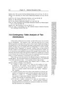
Figure 14.4.1. Example of a contingency table for two nominal variables, here sex and color. The
row and column marginals (totals) are shown. The variables are “nominal,” i.e., the order in which
their values are listed is arbitrary and does not affect the result of the contingency table analysis. If
the ordering of values has some intrinsic meaning, then the variables are “ordinal” or “continuous,” and
correlation techniques (§14.5-§14.6) can be utilized.
A continuous variable can always be made into an ordinal one by binning it
into ranges. If we choose to ignore the ordering of the bins, then we can turn it into
a nominal variable. Nominal variables constitute the lowest type of the hierarchy,
and therefore the most general. For example, a set of several continuous or ordinal
variables can be turned, if crudely, into a single nominal variable, by coarsely
binning each variable and then taking each distinct combination of bin assignments
as a single nominal value. When multidimensional data are sparse, this is often
the only sensible way to proceed.
The remainder of this section will deal with measures of association between
nominal variables. For any pair of nominal variables, the data can be displayed as
a contingency table, a table whose rows are labeled by the values of one nominal
variable, whose columns are labeled by the values of the other nominal variable,
and whose entries are nonnegative integers giving the number of observed events
for each combination of row and column (see Figure 14.4.1). The analysis of

association between nominal variables is thus called contingency table analysis or
crosstabulation analysis.
We will introduce two different approaches. The first approach, based on the
chi-square statistic, does a good job of characterizing the significance of association,
but is only so-so as a measure of the strength (principally because its numerical
values have no very direct interpretations). The second approach, based on the
information-theoreticconcept of entropy, says nothing at all about the significance of
association (use chi-square for that!), but is capable of very elegantly characterizing
the strength of an association already known to be significant.
630
Chapter 14. Statistical Description of Data
Sample page from NUMERICAL RECIPES IN C: THE ART OF SCIENTIFIC COMPUTING (ISBN 0-521-43108-5)
Copyright (C) 1988-1992 by Cambridge University Press.Programs Copyright (C) 1988-1992 by Numerical Recipes Software.
Permission is granted for internet users to make one paper copy for their own personal use. Further reproduction, or any copying of machine-
readable files (including this one) to any servercomputer, is strictly prohibited. To order Numerical Recipes books,diskettes, or CDROMs
visit website or call 1-800-872-7423 (North America only),or send email to (outside North America).
Measures of Association Based on Chi-Square
Some notation first: Let N
ij
denote the number of events that occur with the
first variable x taking on its ith value, and the second variable y taking on its jth
value. Let N denote the total number of events, the sum of all the N
ij
’s. Let N
i·
denote the number of events for which the first variable x takes on its ith value
regardless of the value of y; N
·j
is the number of events with the jth value of y
regardless of x.Sowehave

N
i·
=

j
N
ij
N
·j
=

i
N
ij
N =

i
N
i·
=

j
N
·j
(14.4.1)
N
·j
and N
i·
are sometimes called the row and column totals or marginals, but we

will use these terms cautiously since we can never keep straight which are the rows
and which are the columns!
The null hypothesis is that the two variables x and y have no association. In this
case, the probability of a particular value of x given a particular value of y should
be the same as the probability of that value of x regardless of y. Therefore, in the
null hypothesis, the expected number for any N
ij
, which we will denote n
ij
, can be
calculated from only the row and column totals,
n
ij
N
·j
=
N
i·
N
which implies n
ij
=
N
i·
N
·j
N
(14.4.2)
Notice that if a column or row total is zero, then the expected number for all the
entries in that column or row is also zero; in that case, the never-occurring bin of

x or y should simply be removed from the analysis.
The chi-square statistic is now given by equation (14.3.1), which, in the present
case, is summed over all entries in the table,
χ
2
=

i,j
(N
ij
− n
ij
)
2
n
ij
(14.4.3)
The number of degrees of freedom is equal to the number of entries in the table
(product of its row size and column size) minus the number of constraints that have
arisen from our use of the data themselves to determine the n
ij
. Each row total and
column total is a constraint, except that this overcounts by one, since the total of the
column totals and the total of the row totals both equal N, the total number of data
points. Therefore, if the table is of size I by J, the number of degrees of freedom is
IJ − I − J +1. Equation (14.4.3), along with the chi-square probability function
(§6.2), now give the significance of an association between the variables x and y.
Suppose there is a significant association. How do we quantify its strength, so
that (e.g.) we can compare the strength of one association with another? The idea
here is to find some reparametrization of χ

2
which maps it into some convenient
interval, like 0 to 1, where the result is not dependent on the quantity of data that we
happen to sample, but rather depends only on the underlying populationfrom which
14.4 Contingency Table Analysis of Two Distributions
631
Sample page from NUMERICAL RECIPES IN C: THE ART OF SCIENTIFIC COMPUTING (ISBN 0-521-43108-5)
Copyright (C) 1988-1992 by Cambridge University Press.Programs Copyright (C) 1988-1992 by Numerical Recipes Software.
Permission is granted for internet users to make one paper copy for their own personal use. Further reproduction, or any copying of machine-
readable files (including this one) to any servercomputer, is strictly prohibited. To order Numerical Recipes books,diskettes, or CDROMs
visit website or call 1-800-872-7423 (North America only),or send email to (outside North America).
the data were drawn. There are several different ways of doing this. Two of the
more common are called Cramer’s V and the contingency coefficient C.
The formula for Cramer’s V is
V =

χ
2
N min (I − 1,J−1)
(14.4.4)
where I and J are again the numbers of rows and columns, and N is the total
number of events. Cramer’s V has the pleasant property that it lies between zero
and one inclusive, equals zero when there is no association, and equals one only
when the association is perfect: All the events in any row lie in one unique column,
and vice versa. (In chess parlance, no two rooks, placed on a nonzero table entry,
can capture each other.)
In the case of I = J =2,Cramer’sV is also referred to as the phi statistic.
The contingency coefficient C is defined as
C =


χ
2
χ
2
+ N
(14.4.5)
It also lies between zero and one, but (as is apparent from the formula) it can never
achieve the upper limit. While it can be used to compare the strength of association
of two tables with the same I and J, its upper limit depends on I and J. Therefore
it can never be used to compare tables of different sizes.
The trouble with both Cramer’s V and the contingency coefficient C is that,
when they take on values in between their extremes, there is no very direct
interpretation of what that value means. For example, you are in Las Vegas, and a
friend tells you that there is a small, but significant, association between the color of
a croupier’s eyes and the occurrence of red and black on his roulettewheel. Cramer’s
V is about 0.028, your friend tells you. You know what the usual odds against you
are (because of the green zero and double zero on the wheel). Is this association
sufficient for you to make money? Don’t ask us!
#include <math.h>
#include "nrutil.h"
#define TINY 1.0e-30 A small number.
void cntab1(int **nn, int ni, int nj, float *chisq, float *df, float *prob,
float *cramrv, float *ccc)
Given a two-dimensional contingency table in the form of an integer array
nn[1..ni][1..nj]
,
this routine returns the chi-square
chisq
, the number of degrees of freedom
df

, the significance
level
prob
(small values indicating a significant association), and two measures of association,
Cramer’s V (
cramrv
) and the contingency coefficient C (
ccc
).
{
float gammq(float a, float x);
int nnj,nni,j,i,minij;
float sum=0.0,expctd,*sumi,*sumj,temp;
sumi=vector(1,ni);
sumj=vector(1,nj);
nni=ni; Number of rows
nnj=nj; and columns.
for (i=1;i<=ni;i++) { Get the row totals.
sumi[i]=0.0;
632
Chapter 14. Statistical Description of Data
Sample page from NUMERICAL RECIPES IN C: THE ART OF SCIENTIFIC COMPUTING (ISBN 0-521-43108-5)
Copyright (C) 1988-1992 by Cambridge University Press.Programs Copyright (C) 1988-1992 by Numerical Recipes Software.
Permission is granted for internet users to make one paper copy for their own personal use. Further reproduction, or any copying of machine-
readable files (including this one) to any servercomputer, is strictly prohibited. To order Numerical Recipes books,diskettes, or CDROMs
visit website or call 1-800-872-7423 (North America only),or send email to (outside North America).
for (j=1;j<=nj;j++) {
sumi[i] += nn[i][j];
sum += nn[i][j];
}

if (sumi[i] == 0.0) --nni; Eliminate any zero rows by reducing the num-
ber.}
for (j=1;j<=nj;j++) { Get the column totals.
sumj[j]=0.0;
for (i=1;i<=ni;i++) sumj[j] += nn[i][j];
if (sumj[j] == 0.0) --nnj; Eliminate any zero columns.
}
*df=nni*nnj-nni-nnj+1; Corrected number of degrees of freedom.
*chisq=0.0;
for (i=1;i<=ni;i++) { Do the chi-square sum.
for (j=1;j<=nj;j++) {
expctd=sumj[j]*sumi[i]/sum;
temp=nn[i][j]-expctd;
*chisq += temp*temp/(expctd+TINY); Here TINY guarantees that any
eliminated row or column will
not contribute to the sum.
}
}
*prob=gammq(0.5*(*df),0.5*(*chisq)); Chi-square probability function.
minij = nni < nnj ? nni-1 : nnj-1;
*cramrv=sqrt(*chisq/(sum*minij));
*ccc=sqrt(*chisq/(*chisq+sum));
free_vector(sumj,1,nj);
free_vector(sumi,1,ni);
}
Measures of Association Based on Entropy
Consider the game of “twenty questions,” where by repeated yes/no questions
you try to eliminate all except one correct possibility for an unknown object. Better
yet, consider a generalization of the game, where you are allowed to ask multiple
choice questions as well as binary (yes/no) ones. The categories in your multiple

choice questions are supposed to be mutually exclusive and exhaustive (as are
“yes” and “no”).
The value to you of an answer increases with the number of possibilities that
it eliminates. More specifically, an answer that eliminates all except a fraction p of
the remaining possibilities can be assigned a value − ln p (a positive number, since
p<1). The purpose of the logarithm is to make the value additive, since (e.g.) one
question that eliminates all but 1/6 of the possibilities is considered as good as two
questions that, in sequence, reduce the number by factors 1/2 and 1/3.
So that is the value of an answer; but what is the value of a question? If there
are I possible answers to the question (i =1,...,I)and the fraction of possibilities
consistent with the ith answer is p
i
(with the sum of the p
i
’s equal to one), then the
value of the question is the expectation value of the value of the answer, denoted H,
H = −
I

i=1
p
i
ln p
i
(14.4.6)
In evaluating (14.4.6), note that
lim
p→0
p ln p =0 (14.4.7)