Tài liệu Modeling Of Data part 8 pptx

15.7 Robust Estimation
699
Sample page from NUMERICAL RECIPES IN C: THE ART OF SCIENTIFIC COMPUTING (ISBN 0-521-43108-5)
Copyright (C) 1988-1992 by Cambridge University Press.Programs Copyright (C) 1988-1992 by Numerical Recipes Software.
Permission is granted for internet users to make one paper copy for their own personal use. Further reproduction, or any copying of machine-
readable files (including this one) to any servercomputer, is strictly prohibited. To order Numerical Recipes books,diskettes, or CDROMs
visit website or call 1-800-872-7423 (North America only),or send email to (outside North America).
C
jk
=
M

i=1
1
w
2
i
V
ji
V
ki
(15.6.10)
CITED REFERENCES AND FURTHER READING:
Efron, B. 1982,
The Jackknife, the Bootstrap, and Other Resampling Plans
(Philadelphia:
S.I.A.M.). [1]
Efron, B., and Tibshirani, R. 1986,
Statistical Science
vol. 1, pp. 54–77. [2]
Avni, Y. 1976,

Astrophysical Journal
, vol. 210, pp. 642–646. [3]
Lampton, M., Margon, M., and Bowyer, S. 1976,
Astrophysical Journal
, vol. 208, pp. 177–190.
Brownlee, K.A. 1965,
Statistical Theory and Methodology
, 2nd ed. (New York: Wiley).
Martin, B.R. 1971,
Statistics for Physicists
(New York: Academic Press).
15.7 Robust Estimation
The concept of robustness has been mentioned in passing several times already.
In §14.1 we noted that the median was a more robust estimator of central value than
the mean; in §14.6 it was mentioned that rank correlation is more robust than linear
correlation. The concept of outlier points as exceptions to a Gaussian model for
experimental error was discussed in §15.1.
The term “robust” was coined in statistics by G.E.P. Box in 1953. Various
definitions of greater or lesser mathematical rigor are possible for the term, but in
general, referring to a statistical estimator, it means “insensitive to small departures
from the idealized assumptions for which the estimator is optimized.”
[1,2]
The word
“small” can have two different interpretations, both important: either fractionally
small departures for all data points, or else fractionally large departures for a small
number of data points. It is the latter interpretation, leading to the notion of outlier
points, that is generally the most stressful for statistical procedures.
Statisticianshave developed varioussortsof robust statistical estimators. Many,
if not most, can be grouped in one of three categories.
M-estimates follow from maximum-likelihood arguments very much as equa-

tions (15.1.5) and (15.1.7) followed from equation (15.1.3). M-estimates are usually
the most relevant class for model-fitting, that is, estimation of parameters. We
therefore consider these estimates in some detail below.
L-estimates are “linear combinations of order statistics.” These are most
applicable to estimations of central value and central tendency, though they can
occasionally be applied to some problems in estimation of parameters. Two
“typical” L-estimates will give you the general idea. They are (i) the median, and
(ii) Tukey’s trimean, defined as the weighted average of the first, second, and third
quartile points in a distribution, with weights 1/4, 1/2, and 1/4, respectively.
R-estimates are estimates based on rank tests. For example, the equality or
inequality of two distributions can be estimated by the Wilcoxon test of computing
the mean rank of one distribution in a combined sample of both distributions.
The Kolmogorov-Smirnov statistic (equation 14.3.6) and the Spearman rank-order
700
Chapter 15. Modeling of Data
Sample page from NUMERICAL RECIPES IN C: THE ART OF SCIENTIFIC COMPUTING (ISBN 0-521-43108-5)
Copyright (C) 1988-1992 by Cambridge University Press.Programs Copyright (C) 1988-1992 by Numerical Recipes Software.
Permission is granted for internet users to make one paper copy for their own personal use. Further reproduction, or any copying of machine-
readable files (including this one) to any servercomputer, is strictly prohibited. To order Numerical Recipes books,diskettes, or CDROMs
visit website or call 1-800-872-7423 (North America only),or send email to (outside North America).
narrow
central peak
tail of
outliers
least squares fit
robust straight-line fit
(a)
(b)
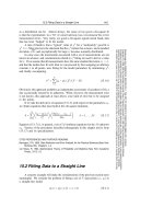
Figure 15.7.1. Examples where robust statistical methods are desirable: (a) A one-dimensional
distribution with atailof outliers; statistical fluctuationsin these outliers can preventaccuratedetermination

of the position of the central peak. (b) A distribution in two dimensions fitted to a straight line; non-robust
techniques such as least-squares fitting can have undesired sensitivity to outlying points.
correlation coefficient (14.6.1) are R-estimates in essence, if not always by formal
definition.
Someotherkindsof robusttechniques, coming from the fields ofoptimalcontrol
and filtering rather than fromthe field of mathematical statistics, are mentioned at the
end of this section. Some examples where robust statistical methods are desirable
are shown in Figure 15.7.1.
Estimation of Parameters by Local M-Estimates
Suppose we know that our measurement errors are not normally distributed.
Then, in deriving a maximum-likelihoodformula for the estimated parameters a in a
model y(x; a), we would write instead of equation (15.1.3)
P =
N

i=1
{exp [−ρ(y
i
,y{x
i
;a})] ∆y} (15.7.1)
15.7 Robust Estimation
701
Sample page from NUMERICAL RECIPES IN C: THE ART OF SCIENTIFIC COMPUTING (ISBN 0-521-43108-5)
Copyright (C) 1988-1992 by Cambridge University Press.Programs Copyright (C) 1988-1992 by Numerical Recipes Software.
Permission is granted for internet users to make one paper copy for their own personal use. Further reproduction, or any copying of machine-
readable files (including this one) to any servercomputer, is strictly prohibited. To order Numerical Recipes books,diskettes, or CDROMs
visit website or call 1-800-872-7423 (North America only),or send email to (outside North America).
where the function ρ is the negative logarithm of the probability density. Taking the
logarithm of (15.7.1) analogously with (15.1.4), we find that we want to minimize

the expression
N

i=1
ρ(y
i
,y{x
i
;a})(15.7.2)
Very often, it is the case that the function ρ depends not independently on its
two arguments, measured y
i
and predicted y(x
i
), but only on their difference, at least
if scaled by some weight factors σ
i
which we are able to assign to each point. In this
case the M-estimate is said to be local, and we can replace (15.7.2) by theprescription
minimize over a
N

i=1
ρ

y
i
− y(x
i
; a)

σ
i

(15.7.3)
where the function ρ(z) is a function of a single variable z ≡ [y
i
− y(x
i
)]/σ
i
.
If we now define the derivative of ρ(z) to be a function ψ(z),
ψ(z) ≡
dρ(z)
dz
(15.7.4)
then the generalization of (15.1.7) to the case of a general M-estimate is
0=
N

i=1
1
σ
i
ψ

y
i
− y(x
i

)
σ
i

∂y(x
i
;a)
∂a
k

k =1,...,M (15.7.5)
If you compare (15.7.3) to (15.1.3), and (15.7.5) to (15.1.7), you see at once
that the specialization for normally distributed errors is
ρ(z)=
1
2
z
2
ψ(z)=z (normal) (15.7.6)
If the errors are distributed as a double or two-sided exponential, namely
Prob {y
i
− y(x
i
)}∼exp

−





y
i
− y(x
i
)
σ
i





(15.7.7)
then, by contrast,
ρ(x)=|z| ψ(z)=sgn(z) (double exponential) (15.7.8)
Comparing to equation (15.7.3), we see that in this case the maximum likelihood
estimator is obtained by minimizing the mean absolute deviation, rather than the
mean square deviation. Here the tails of the distribution, although exponentially
decreasing, are asymptotically much larger than any corresponding Gaussian.
A distribution with even more extensive — therefore sometimes even more
realistic — tails is the Cauchy or Lorentzian distribution,
Prob {y
i
− y(x
i
)}∼
1
1+
1

2

y
i
−y(x
i
)
σ
i

2
(15.7.9)
702
Chapter 15. Modeling of Data
Sample page from NUMERICAL RECIPES IN C: THE ART OF SCIENTIFIC COMPUTING (ISBN 0-521-43108-5)
Copyright (C) 1988-1992 by Cambridge University Press.Programs Copyright (C) 1988-1992 by Numerical Recipes Software.
Permission is granted for internet users to make one paper copy for their own personal use. Further reproduction, or any copying of machine-
readable files (including this one) to any servercomputer, is strictly prohibited. To order Numerical Recipes books,diskettes, or CDROMs
visit website or call 1-800-872-7423 (North America only),or send email to (outside North America).
This implies
ρ(z)=log

1+
1
2
z
2

ψ(z)=
z

1+
1
2
z
2
(Lorentzian) (15.7.10)
Notice that the ψ function occurs as a weighting function in the generalized
normal equations (15.7.5). For normally distributed errors, equation (15.7.6) says
that the more deviant the points, the greater the weight. By contrast, when tails are
somewhat more prominent, as in (15.7.7), then (15.7.8) says that all deviant points
get the same relative weight, with only the sign information used. Finally, when
the tails are even larger, (15.7.10) says the ψ increases with deviation, then starts
decreasing, so that very deviant points — the true outliers — are not counted at all
in the estimation of the parameters.
This general idea, that the weight given individual points should first increase
with deviation, then decrease, motivates some additional prescriptions for ψ which
do not especially correspond to standard, textbook probability distributions. Two
examples are
Andrew’s sine
ψ(z)=

sin(z/c)
0
|z| <cπ
|z|>cπ
(15.7.11)
If the measurement errors happen to be normal after all, with standard deviations σ
i
,
then it can be shown that the optimal value for the constant c is c =2.1.

Tukey’s biweight
ψ(z)=

z(1 − z
2
/c
2
)
2
0
|z| <c
|z|>c
(15.7.12)
where the optimal value of c for normal errors is c =6.0.
Numerical Calculation of M-Estimates
To fit a model by means of an M-estimate, you first decide which M-estimate
you want, that is, which matching pair ρ, ψ you want to use. We rather like
(15.7.8) or (15.7.10).
You then have to make an unpleasant choice between two fairly difficult
problems. Either find the solution of the nonlinear set of M equations (15.7.5), or
else minimize the single function in M variables (15.7.3).
Notice that the function (15.7.8) has a discontinuous ψ, and a discontinuous
derivative for ρ. Such discontinuities frequently wreak havoc on both general
nonlinear equation solvers and general function minimizing routines. You might
now think of rejecting (15.7.8) in favor of (15.7.10), which is smoother. However,
you will find that the latter choice is also bad news for many general equation solving
or minimization routines: small changes in the fitted parameters can drive ψ(z)
off its peak into one or the other of its asymptotically small regimes. Therefore,
different terms in the equation spring into or out of action (almost as bad as analytic
discontinuities).

Don’t despair. If your computer budget (or, for personal computers, patience)
is up to it, this is an excellent application for the downhill simplex minimization
15.7 Robust Estimation
703
Sample page from NUMERICAL RECIPES IN C: THE ART OF SCIENTIFIC COMPUTING (ISBN 0-521-43108-5)
Copyright (C) 1988-1992 by Cambridge University Press.Programs Copyright (C) 1988-1992 by Numerical Recipes Software.
Permission is granted for internet users to make one paper copy for their own personal use. Further reproduction, or any copying of machine-
readable files (including this one) to any servercomputer, is strictly prohibited. To order Numerical Recipes books,diskettes, or CDROMs
visit website or call 1-800-872-7423 (North America only),or send email to (outside North America).
algorithmexemplified in amoeba §10.4 or amebsa in §10.9. Those algorithms make
no assumptions about continuity;they just ooze downhill and will work for virtually
any sane choice of the function ρ.
It is very much to your (financial) advantage to find good starting values,
however. Often this is done by first fitting the model by the standard χ
2
(nonrobust)
techniques, e.g., as described in §15.4 or §15.5. The fitted parameters thus obtained
are then used as starting values in amoeba, now using the robust choice of ρ and
minimizing the expression (15.7.3).
Fitting a Line by Minimizing Absolute Deviation
Occasionally there is a special case that happens to be much easier than is
suggested by the general strategy outlined above. The case of equations (15.7.7)–
(15.7.8), when the model is a simple straight line
y(x; a, b)=a+bx (15.7.13)
and where the weights σ
i
are all equal, happens to be such a case. The problem is
precisely the robust version of the problem posed in equation (15.2.1) above, namely
fit a straight line through a set of data points. The merit function to be minimized is
N


i=1
|y
i
− a − bx
i
| (15.7.14)
rather than the χ
2
given by equation (15.2.2).
The key simplification is based on the following fact: The median c
M
of a set
of numbers c
i
is also that value which minimizes the sum of the absolute deviations

i
|c
i
− c
M
|
(Proof: Differentiate the above expression with respect to c
M
and set it to zero.)
It follows that, for fixed b, the value of a that minimizes (15.7.14) is
a = median {y
i
− bx

i
} (15.7.15)
Equation (15.7.5) for the parameter b is
0=
N

i=1
x
i
sgn(y
i
− a − bx
i
)(15.7.16)
(where sgn(0) is to be interpreted as zero). If we replace a in this equation by the
implied function a(b) of (15.7.15), then we are left with an equation in a single
variable which can be solved by bracketing and bisection, as described in §9.1.
(In fact, it is dangerous to use any fancier method of root-finding, because of the
discontinuities in equation 15.7.16.)
Here is a routine that does all this. It calls select (§8.5) to find the median.
The bracketing and bisection are built in to the routine, as is the χ
2
solution that
generates the initial guesses for a and b. Notice that the evaluation of the right-hand
side of (15.7.16) occurs in the function rofunc, with communication via global
(top-level) variables.