Statistical Description of Data part 8

14.7 Do Two-Dimensional Distributions Differ?
645
Sample page from NUMERICAL RECIPES IN C: THE ART OF SCIENTIFIC COMPUTING (ISBN 0-521-43108-5)
Copyright (C) 1988-1992 by Cambridge University Press.Programs Copyright (C) 1988-1992 by Numerical Recipes Software.
Permission is granted for internet users to make one paper copy for their own personal use. Further reproduction, or any copying of machine-
readable files (including this one) to any servercomputer, is strictly prohibited. To order Numerical Recipes books,diskettes, or CDROMs
visit website or call 1-800-872-7423 (North America only),or send email to (outside North America).
li=l/j; decoding its row
lj=l-j*li; and column.
mm=(m1=li-ki)*(m2=lj-kj);
pairs=tab[ki+1][kj+1]*tab[li+1][lj+1];
if (mm) { Not a tie.
en1 += pairs;
en2 += pairs;
s += (mm > 0 ? pairs : -pairs); Concordant, or discordant.
} else {
if (m1) en1 += pairs;
if (m2) en2 += pairs;
}
}
}
*tau=s/sqrt(en1*en2);
svar=(4.0*points+10.0)/(9.0*points*(points-1.0));
*z=(*tau)/sqrt(svar);
*prob=erfcc(fabs(*z)/1.4142136);
}
CITED REFERENCES AND FURTHER READING:
Lehmann, E.L. 1975,
Nonparametrics: Statistical Methods Based on Ranks
(San Francisco:
Holden-Day).

Downie, N.M., and Heath, R.W. 1965,
Basic Statistical Methods
, 2nd ed. (New York: Harper &
Row), pp. 206–209.
Norusis, M.J. 1982,
SPSS Introductory Guide: Basic Statistics and Operations
; and 1985,
SPSS-
X Advanced Statistics Guide
(New York: McGraw-Hill).
14.7 Do Two-Dimensional Distributions Differ?
We here discuss a useful generalization of the K–S test (§14.3) to two-dimensional
distributions. This generalization is due to Fasano and Franceschini
[1]
,avariantonan
earlier idea due to Peacock
[2]
.
In a two-dimensional distribution, each data point is characterized by an (x, y) pair of
values. An example near to our hearts is that each of the 19 neutrinos that were detected
from Supernova 1987A is characterized by a time t
i
andbyanenergyE
i
(see
[3]
). We
might wish to know whether these measured pairs (t
i
,E

i
),i=1...19 are consistent with a
theoretical model that predicts neutrino flux as a function of both time and energy — that is,
a two-dimensional probability distribution in the (x, y) [here, (t, E)] plane. That would be a
one-sample test. Or, given two sets of neutrino detections, from two comparable detectors,
we might want to know whether they are compatible with each other, a two-sample test.
In the spirit of the tried-and-true, one-dimensional K–S test, we want to range over
the (x, y) plane in search of some kind of maximum cumulative difference between two
two-dimensional distributions. Unfortunately, cumulative probability distribution is not
well-defined in more than one dimension! Peacock’s insight was that a good surrogate is
the integrated probability in each of four natural quadrants around a given point (x
i
,y
i
),
namely the total probabilities (or fraction of data) in (x>x
i
,y > y
i
), (x<x
i
,y > y
i
),
(x<x
i
,y < y
i
), (x>x
i

,y < y
i
). The two-dimensional K–S statistic D is now taken
to be the maximum difference (ranging both over data points and over quadrants) of the
corresponding integrated probabilities. When comparing two data sets, the value of D may
depend on which data set is ranged over. In that case, define an effective D as the average
646
Chapter 14. Statistical Description of Data
Sample page from NUMERICAL RECIPES IN C: THE ART OF SCIENTIFIC COMPUTING (ISBN 0-521-43108-5)
Copyright (C) 1988-1992 by Cambridge University Press.Programs Copyright (C) 1988-1992 by Numerical Recipes Software.
Permission is granted for internet users to make one paper copy for their own personal use. Further reproduction, or any copying of machine-
readable files (including this one) to any servercomputer, is strictly prohibited. To order Numerical Recipes books,diskettes, or CDROMs
visit website or call 1-800-872-7423 (North America only),or send email to (outside North America).
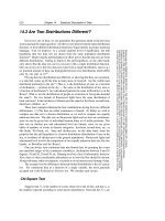
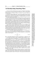
−3 −2 −1 0123
−3
−2
−1
0
1
2
3
.11
|
.09
.65
|
.26
.12
|
.09

.12
|
.56
Figure 14.7.1. Two-dimensional distributions of 65 triangles and 35 squares. The two-dimensional K–S
test finds that point one of whose quadrants (shown by dotted lines) maximizes the difference between
fraction of triangles and fraction of squares. Then, equation (14.7.1) indicates whether the difference is
statistically significant, i.e., whetherthetrianglesand squaresmusthave differentunderlyingdistributions.
of the two values obtained. If you are confused at this point about the exact definition of D,
don’t fret; the accompanying computer routines amount to a precise algorithmic definition.
Figure 14.7.1 gives a feeling for what is going on. The 65 triangles and 35 squares seem
to have somewhat different distributions in the plane. The dotted lines are centered on the
triangle that maximizes the D statistic; the maximum occurs in the upper-left quadrant. That
quadrant contains only 0.12 of all the triangles, but it contains 0.56 of all the squares. The
value of D is thus 0.44. Is this statistically significant?
Even for fixed sample sizes, it is unfortunately not rigorously true that the distribution
of D in the null hypothesis is independent of the shape of the two-dimensional distribution.
In this respect the two-dimensional K–S test is not as natural as its one-dimensional parent.
However, extensive Monte Carlo integrations have shown that the distribution of the two-
dimensional D is very nearly identical for even quite different distributions, as long as they
have the same coefficient of correlation r, defined in the usual way by equation (14.5.1). In
their paper, Fasano and Franceschini tabulate Monte Carlo results for (what amounts to) the
distribution of D as a function of (of course) D,samplesizeN, and coefficient of correlation
r. Analyzing their results, one finds that the significance levels for the two-dimensional K–S
test can be summarized by the simple, though approximate, formulas,
Probability (D>observed )=Q
KS

√
ND
1+

√
1−r
2
(0.25 − 0.75/
√
N)

(14.7.1)
14.7 Do Two-Dimensional Distributions Differ?
647
Sample page from NUMERICAL RECIPES IN C: THE ART OF SCIENTIFIC COMPUTING (ISBN 0-521-43108-5)
Copyright (C) 1988-1992 by Cambridge University Press.Programs Copyright (C) 1988-1992 by Numerical Recipes Software.
Permission is granted for internet users to make one paper copy for their own personal use. Further reproduction, or any copying of machine-
readable files (including this one) to any servercomputer, is strictly prohibited. To order Numerical Recipes books,diskettes, or CDROMs
visit website or call 1-800-872-7423 (North America only),or send email to (outside North America).
for the one-sample case, and the same for the two-sample case, but with
N =
N
1
N
2
N
1
+ N
2
. (14.7.2)
The above formulas are accurate enough when N
>
∼
20, and when the indicated

probability (significance level) is less than (more significant than) 0.20 or so. When the
indicated probability is > 0.20, its value may not be accurate, but the implication that the
data and model (or two data sets) are not significantly different is certainly correct. Notice
that in the limit of r → 1 (perfect correlation), equations (14.7.1) and (14.7.2) reduce to
equations (14.3.9) and (14.3.10): The two-dimensional data lie on a perfect straight line, and
the two-dimensional K–S test becomes a one-dimensional K–S test.
The significance level for the data in Figure 14.7.1, by the way, is about 0.001. This
establishes to a near-certainty that the triangles and squares were drawn from different
distributions. (As in fact they were.)
Of course, if you do not want to rely on the Monte Carlo experiments embodied in
equation (14.7.1), you can do your own: Generate a lot of synthetic data sets from your
model, each one with the same number of points as the real data set. Compute D for each
synthetic data set, using the accompanying computer routines (but ignoring their calculated
probabilities), and count what fraction of the time these synthetic D’s exceed the D from the
real data. That fraction is your significance.
One disadvantage of the two-dimensional tests, by comparison with their one-
dimensional progenitors, is that the two-dimensional tests require of order N
2
operations:
Two nested loops of order N take the place of an N log N sort. For small computers, this
restricts the usefulness of the tests to N less than several thousand.
We now give computer implementations. The one-sample case is embodied in the
routine ks2d1s (that is, 2-dimensions, 1-sample). This routine calls a straightforward utility
routine quadct to count points in the four quadrants, and it calls a user-supplied routine
quadvl that must be capable of returning the integrated probability of an analytic model in
each of four quadrants around an arbitrary (x, y) point. A trivial sample quadvl is shown;
realistic quadvls can be quite complicated, often incorporating numerical quadratures over
analytic two-dimensional distributions.
#include <math.h>
#include "nrutil.h"

void ks2d1s(float x1[], float y1[], unsigned long n1,
void (*quadvl)(float, float, float *, float *, float *, float *),
float *d1, float *prob)
Two-dimensional Kolmogorov-Smirnov test of one sample against a model. Given the x and y
coordinates of
n1
data points in arrays
x1[1..n1]
and
y1[1..n1]
, and given a user-supplied
function
quadvl
that exemplifies the model, this routine returns the two-dimensional K-S
statistic as
d1
, and its significance level as
prob
. Small values of
prob
show that the sample
is significantly different from the model. Note that the test is slightly distribution-dependent,
so
prob
is only an estimate.
{
void pearsn(float x[], float y[], unsigned long n, float *r, float *prob,
float *z);
float probks(float alam);
void quadct(float x, float y, float xx[], float yy[], unsigned long nn,

float *fa, float *fb, float *fc, float *fd);
unsigned long j;
float dum,dumm,fa,fb,fc,fd,ga,gb,gc,gd,r1,rr,sqen;
*d1=0.0;
for (j=1;j<=n1;j++) { Loop over the data points.
quadct(x1[j],y1[j],x1,y1,n1,&fa,&fb,&fc,&fd);
(*quadvl)(x1[j],y1[j],&ga,&gb,&gc,&gd);
*d1=FMAX(*d1,fabs(fa-ga));
*d1=FMAX(*d1,fabs(fb-gb));
*d1=FMAX(*d1,fabs(fc-gc));
648
Chapter 14. Statistical Description of Data
Sample page from NUMERICAL RECIPES IN C: THE ART OF SCIENTIFIC COMPUTING (ISBN 0-521-43108-5)
Copyright (C) 1988-1992 by Cambridge University Press.Programs Copyright (C) 1988-1992 by Numerical Recipes Software.
Permission is granted for internet users to make one paper copy for their own personal use. Further reproduction, or any copying of machine-
readable files (including this one) to any servercomputer, is strictly prohibited. To order Numerical Recipes books,diskettes, or CDROMs
visit website or call 1-800-872-7423 (North America only),or send email to (outside North America).
*d1=FMAX(*d1,fabs(fd-gd));
For both the sample and the model, the distribution is integrated in each of four
quadrants, and the maximum difference is saved.
}
pearsn(x1,y1,n1,&r1,&dum,&dumm); Get the linear correlation coefficient r1.
sqen=sqrt((double)n1);
rr=sqrt(1.0-r1*r1);
Estimate the probability using the K-S probability function probks.
*prob=probks(*d1*sqen/(1.0+rr*(0.25-0.75/sqen)));
}
void quadct(float x, float y, float xx[], float yy[], unsigned long nn,
float *fa, float *fb, float *fc, float *fd)
Givenanorigin(

x
,
y
), and an array of
nn
points with coordinates
xx[1..nn]
and
yy[1..nn]
,
count how many of them are in each quadrant around the origin, and return the normalized
fractions. Quadrants are labeled alphabetically, counterclockwise from the upper right. Used
by
ks2d1s
and
ks2d2s
.
{
unsigned long k,na,nb,nc,nd;
float ff;
na=nb=nc=nd=0;
for (k=1;k<=nn;k++) {
if (yy[k] > y) {
xx[k] > x ? ++na : ++nb;
} else {
xx[k] > x ? ++nd : ++nc;
}
}
ff=1.0/nn;
*fa=ff*na;

*fb=ff*nb;
*fc=ff*nc;
*fd=ff*nd;
}
#include "nrutil.h"
void quadvl(float x, float y, float *fa, float *fb, float *fc, float *fd)
This is a sample of a user-supplied routine to be used with
ks2d1s
. In this case, the model
distribution is uniform inside the square −1 <x<1,−1<y<1. In general this routine
should return, for any point (
x
,
y
), the fraction of the total distribution in each of the four
quadrants around that point. The fractions,
fa
,
fb
,
fc
,and
fd
, must add up to 1. Quadrants
are alphabetical, counterclockwise from the upper right.
{
float qa,qb,qc,qd;
qa=FMIN(2.0,FMAX(0.0,1.0-x));
qb=FMIN(2.0,FMAX(0.0,1.0-y));
qc=FMIN(2.0,FMAX(0.0,x+1.0));

qd=FMIN(2.0,FMAX(0.0,y+1.0));
*fa=0.25*qa*qb;
*fb=0.25*qb*qc;
*fc=0.25*qc*qd;
*fd=0.25*qd*qa;
}
The routine ks2d2s is thetwo-sample case of the two-dimensional K–S test. It alsocalls
quadct, pearsn,andprobks. Being a two-sample test, it does not need an analytic model.
14.7 Do Two-Dimensional Distributions Differ?
649
Sample page from NUMERICAL RECIPES IN C: THE ART OF SCIENTIFIC COMPUTING (ISBN 0-521-43108-5)
Copyright (C) 1988-1992 by Cambridge University Press.Programs Copyright (C) 1988-1992 by Numerical Recipes Software.
Permission is granted for internet users to make one paper copy for their own personal use. Further reproduction, or any copying of machine-
readable files (including this one) to any servercomputer, is strictly prohibited. To order Numerical Recipes books,diskettes, or CDROMs
visit website or call 1-800-872-7423 (North America only),or send email to (outside North America).
#include <math.h>
#include "nrutil.h"
void ks2d2s(float x1[], float y1[], unsigned long n1, float x2[], float y2[],
unsigned long n2, float *d, float *prob)
Two-dimensional Kolmogorov-Smirnov test on two samples. Given the x and y coordinates of
thefirstsampleas
n1
values in arrays
x1[1..n1]
and
y1[1..n1]
, and likewise for the second
sample,
n2
values in arrays

x2
and
y2
, this routine returns the two-dimensional, two-sample
K-S statistic as
d
, and its significance level as
prob
. Small values of
prob
show that the
two samples are significantly different. Note that the test is slightly distribution-dependent, so
prob
is only an estimate.
{
void pearsn(float x[], float y[], unsigned long n, float *r, float *prob,
float *z);
float probks(float alam);
void quadct(float x, float y, float xx[], float yy[], unsigned long nn,
float *fa, float *fb, float *fc, float *fd);
unsigned long j;
float d1,d2,dum,dumm,fa,fb,fc,fd,ga,gb,gc,gd,r1,r2,rr,sqen;
d1=0.0;
for (j=1;j<=n1;j++) { First, use points in the first sample as ori-
gins.quadct(x1[j],y1[j],x1,y1,n1,&fa,&fb,&fc,&fd);
quadct(x1[j],y1[j],x2,y2,n2,&ga,&gb,&gc,&gd);
d1=FMAX(d1,fabs(fa-ga));
d1=FMAX(d1,fabs(fb-gb));
d1=FMAX(d1,fabs(fc-gc));
d1=FMAX(d1,fabs(fd-gd));

}
d2=0.0;
for (j=1;j<=n2;j++) { Then, use points in the second sample as
origins.quadct(x2[j],y2[j],x1,y1,n1,&fa,&fb,&fc,&fd);
quadct(x2[j],y2[j],x2,y2,n2,&ga,&gb,&gc,&gd);
d2=FMAX(d2,fabs(fa-ga));
d2=FMAX(d2,fabs(fb-gb));
d2=FMAX(d2,fabs(fc-gc));
d2=FMAX(d2,fabs(fd-gd));
}
*d=0.5*(d1+d2); Average the K-S statistics.
sqen=sqrt(n1*n2/(double)(n1+n2));
pearsn(x1,y1,n1,&r1,&dum,&dumm); Get the linear correlation coefficient for each
sample.pearsn(x2,y2,n2,&r2,&dum,&dumm);
rr=sqrt(1.0-0.5*(r1*r1+r2*r2));
Estimate the probability using the K-S probability function probks.
*prob=probks(*d*sqen/(1.0+rr*(0.25-0.75/sqen)));
}
CITED REFERENCES AND FURTHER READING:
Fasano, G. and Franceschini, A. 1987,
Monthly Notices of the Royal Astronomical Society
,
vol. 225, pp. 155–170. [1]
Peacock, J.A. 1983,
Monthly Notices of the Royal Astronomical Society
, vol. 202, pp. 615–627.
[2]
Spergel, D.N., Piran, T., Loeb, A., Goodman, J., and Bahcall, J.N. 1987,
Science
, vol. 237,

pp. 1471–1473. [3]