Tài liệu Evaluation of Functions part 12 doc

198
Chapter 5. Evaluation of Functions
Sample page from NUMERICAL RECIPES IN C: THE ART OF SCIENTIFIC COMPUTING (ISBN 0-521-43108-5)
Copyright (C) 1988-1992 by Cambridge University Press.Programs Copyright (C) 1988-1992 by Numerical Recipes Software.
Permission is granted for internet users to make one paper copy for their own personal use. Further reproduction, or any copying of machine-
readable files (including this one) to any servercomputer, is strictly prohibited. To order Numerical Recipes books,diskettes, or CDROMs
visit website or call 1-800-872-7423 (North America only),or send email to (outside North America).
void pcshft(float a, float b, float d[], int n)
Polynomial coefficient shift. Given a coefficient array
d[0..n-1]
, this routine generates a
coefficient array g
[0..n-1]
such that

n-1
k=0
d
k
y
k
=

n-1
k=0
g
k
x
k
,wherexand y are related
by (5.8.10), i.e., the interval −1 <y<1is mapped to the interval

a
<x<
b
. The array
g is returned in
d
.
{
int k,j;
float fac,cnst;
cnst=2.0/(b-a);
fac=cnst;
for (j=1;j<n;j++) { First we rescale by the factor const...
d[j] *= fac;
fac *= cnst;
}
cnst=0.5*(a+b); ...which is then redefined as the desired shift.
for (j=0;j<=n-2;j++) We accomplish the shift by synthetic division. Synthetic
division is a miracle of high-school algebra. If you
never learned it, go do so. You won’t be sorry.
for (k=n-2;k>=j;k--)
d[k] -= cnst*d[k+1];
}
CITED REFERENCES AND FURTHER READING:
Acton, F.S. 1970,
Numerical Methods That Work
; 1990, corrected edition (Washington: Mathe-
matical Association of America), pp. 59, 182–183 [synthetic division].
5.11 Economization of Power Series
One particular application of Chebyshev methods, the economization of power series,is

an occasionally useful technique, with a flavor of getting something for nothing.
Suppose that you are already computing a function by the use of a convergent power
series, for example
f(x) ≡ 1 −
x
3!
+
x
2
5!
−
x
3
7!
+ ··· (5.11.1)
(This function is actually sin(
√
x)/
√
x, but pretend you don’t know that.) You might be
doing a problem that requires evaluating the series many times in some particular interval, say
[0, (2π)
2
]. Everything is fine, except that the series requires a large number of terms before
its error (approximated by the first neglected term, say) is tolerable. In our example, with
x =(2π)
2
, the first term smaller than 10
−7
is x

13
/(27!). This then approximates the error
of the finite series whose last term is x
12
/(25!).
Notice that because of the large exponent in x
13
, the error is much smaller than 10
−7
everywherein the interval except at the very largest values of x. This is the feature that allows
“economization”: if we are willing to let the error elsewhere in the interval rise to about the
same value that the first neglected term has at the extreme end of the interval, then we can
replace the 13-term series by one that is significantly shorter.
Here are the steps for doing so:
1. Change variables from x to y, as in equation (5.8.10), to map the x interval into
−1 ≤ y ≤ 1.
2. Find the coefficients of the Chebyshev sum (like equation 5.8.8) that exactly equals your
truncated power series (the one with enough terms for accuracy).
3. Truncate this Chebyshevseries to a smaller number of terms, using the coefficientof the
first neglected Chebyshev polynomial as an estimate of the error.
5.11 Economization of Power Series
199
Sample page from NUMERICAL RECIPES IN C: THE ART OF SCIENTIFIC COMPUTING (ISBN 0-521-43108-5)
Copyright (C) 1988-1992 by Cambridge University Press.Programs Copyright (C) 1988-1992 by Numerical Recipes Software.
Permission is granted for internet users to make one paper copy for their own personal use. Further reproduction, or any copying of machine-
readable files (including this one) to any servercomputer, is strictly prohibited. To order Numerical Recipes books,diskettes, or CDROMs
visit website or call 1-800-872-7423 (North America only),or send email to (outside North America).
4. Convert back to a polynomial in y.
5. Change variables back to x.
All of these steps can be done numerically, given the coefficients of the original power

series expansion. The first step is exactly the inverse of the routine pcshft (§5.10), which
mapped a polynomial from y (in the interval [−1, 1])tox(in the interval [a, b]). But since
equation (5.8.10) is a linear relation between x and y, one can also use pcshft for the
inverse. The inverse of
pcshft(a,b,d,n)
turns out to be (you can check this)
pcshft

−2 − b − a
b − a
,
2− b − a
b − a
,d,n

The secondstep requires the inverse operationto that done by the routine chebpc(which
took Chebyshev coefficients into polynomial coefficients). The following routine, pccheb,
accomplishes this, using the formula
[1]
x
k
=
1
2
k−1

T
k
(x)+


k
1

T
k−2
(x)+

k
2

T
k−4
(x)+···

(5.11.2)
where the last term depends on whether k is even or odd,
···+

k
(k−1)/2

T
1
(x)(kodd), ···+
1
2

k
k/2


T
0
(x)(keven). (5.11.3)
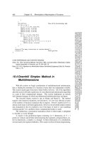
void pccheb(float d[], float c[], int n)
Inverse of routine
chebpc
: given an array of polynomial coefficients
d[0..n-1]
, returns an
equivalent array of Chebyshev coefficients
c[0..n-1]
.
{
int j,jm,jp,k;
float fac,pow;
pow=1.0; Will be powers of 2.
c[0]=2.0*d[0];
for (k=1;k<n;k++) { Loop over orders of x in the polynomial.
c[k]=0.0; Zero corresponding order of Chebyshev.
fac=d[k]/pow;
jm=k;
jp=1;
for (j=k;j>=0;j-=2,jm--,jp++) {
Increment this and lower orders of Chebyshev with the combinatorial coefficent times
d[k]; see text for formula.
c[j] += fac;
fac *= ((float)jm)/((float)jp);
}
pow += pow;
}

}
The fourth and fifth steps are accomplished by the routines chebpc and pcshft,
respectively. Here is how the procedure looks all together:
200
Chapter 5. Evaluation of Functions
Sample page from NUMERICAL RECIPES IN C: THE ART OF SCIENTIFIC COMPUTING (ISBN 0-521-43108-5)
Copyright (C) 1988-1992 by Cambridge University Press.Programs Copyright (C) 1988-1992 by Numerical Recipes Software.
Permission is granted for internet users to make one paper copy for their own personal use. Further reproduction, or any copying of machine-
readable files (including this one) to any servercomputer, is strictly prohibited. To order Numerical Recipes books,diskettes, or CDROMs
visit website or call 1-800-872-7423 (North America only),or send email to (outside North America).
#define NFEW ..
#define NMANY ..
float *c,*d,*e,a,b;
Economize NMANY power series coefficients e[0..NMANY-1] in the range (a, b) into NFEW
coefficients d[0..NFEW-1].
c=vector(0,NMANY-1);
d=vector(0,NFEW-1);
e=vector(0,NMANY-1);
pcshft((-2.0-b-a)/(b-a),(2.0-b-a)/(b-a),e,NMANY);
pccheb(e,c,NMANY);
...
Here one would normally examine the Chebyshev coefficients c[0..NMANY-1] to decide
how small NFEW can be.
chebpc(c,d,NFEW);
pcshft(a,b,d,NFEW);
In our example, by the way, the 8th through 10th Chebyshev coefficients turn out to
be on the order of −7 × 10
−6
, 3 × 10
−7

,and−9×10
−9
, so reasonable truncations (for
single precision calculations) are somewhere in this range, yielding a polynomial with 8 –
10 terms instead of the original 13.
Replacing a 13-term polynomial with a (say) 10-term polynomial without any loss of
accuracy — that does seem to be getting something for nothing. Is there some magic in
this technique? Not really. The 13-term polynomial defined a function f (x). Equivalent to
economizing the series, we could instead have evaluated f(x) at enough points to construct
its Chebyshev approximation in the interval of interest, by the methods of §5.8. We would
have obtained just the same lower-order polynomial. The principal lesson is that the rate
of convergence of Chebyshev coefficients has nothing to do with the rate of convergence of
power series coefficients; and it is the former that dictates the number of terms needed in a
polynomial approximation. A function might have a divergent power series in some region
of interest, but if the function itself is well-behaved, it will have perfectly good polynomial
approximations. These can be found by the methods of §5.8, but not by economization of
series. There is slightly less to economization of series than meets the eye.
CITED REFERENCES AND FURTHER READING:
Acton, F.S. 1970,
Numerical Methods That Work
; 1990, corrected edition (Washington: Mathe-
matical Association of America), Chapter 12.
Arfken, G. 1970,
Mathematical Methods for Physicists
, 2nd ed. (New York: Academic Press),
p. 631. [1]
5.12 Pad
´
e Approximants
A Pad´e approximant, so called, is that rational function (of a specified order) whose

power series expansion agrees with a given power series to the highest possible order. If
the rational function is
R(x) ≡
M

k=0
a
k
x
k
1+
N

k=1
b
k
x
k
(5.12.1)