Tài liệu RF và mạch lạc lò vi sóng P3 docx

3
TRANSMISSION LINES
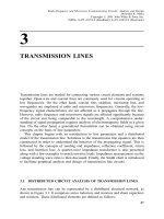
Transmission lines are needed for connecting various circuit elements and systems
together. Open-wire and coaxial lines are commonly used for circuits operating at
low frequencies. On the other hand, coaxial line, stripline, microstrip line, and
waveguides are employed at radio and microwave frequencies. Generally, the low-
frequency signal characteristics are not affected as it propagates through the line.
However, radio frequency and microwave signals are affected signi®cantly because
of the circuit size being comparable to the wavelength. A comprehensive under-
standing of signal propagation requires analysis of electromagnetic ®elds in a given
line. On the other hand, a generalized formulation can be obtained using circuit
concepts on the basis of line parameters.
This chapter begins with an introduction to line parameters and a distributed
model of the transmission line. Solutions to the transmission line equation are then
constructed in order to understand the behavior of the propagating signal. This is
followed by the concepts of sending end impedance, re¯ection coef®cient, return
loss, and insertion loss. A quarter-wave impedance transformer is also presented
along with a few examples to match resistive loads. Impedance measurement via the
voltage standing wave ratio is then discussed. Finally, the Smith chart is introduced
to facilitate graphical analysis and design of transmission line circuits.
3.1 DISTRIBUTED CIRCUIT ANALYSIS OF TRANSMISSION LINES
Any transmission line can be represented by a distributed electrical network, as
shown in Figure 3.1. It comprises series inductors and resistors and shunt capacitors
and resistors. These distributed elements are de®ned as follows:
57
Radio-Frequency and Microwave Communication Circuits: Analysis and Design
Devendra K. Misra
Copyright # 2001 John Wiley & Sons, Inc.
ISBNs: 0-471-41253-8 (Hardback); 0-471-22435-9 (Electronic)
L  Inductance per unit length (H=m)
R  Resistance per unit length (ohm=m)

C  Capacitance per unit length (F=m)
G  Conductance per unit length (S=m)
L, R, C, and G are called the line parameters, which are determined theoretically by
electromagnetic ®eld analysis of the transmission line. These parameters are
in¯uenced by their cross-section geometry and the electrical characteristics of
their constituents. For example, if a line is made up of an ideal dielectric and a
perfect conductor then its R and G will be zero. If it is a coaxial cable with inner and
outer radii a and b, respectively, as shown in Figure 3.2, then,
C 
55:63e
r
lnb=a
pF=m 3:1:1
and,
L  200 lnb=a nH=m 3:1:2
Figure 3.1 Distributed network model of a transmission line.
Figure 3.2 Coaxial line geometry.
58
TRANSMISSION LINES
where e
r
is the dielectric constant of the material between two coaxial conductors of
the line.
If the coaxial line has small losses due to imperfect conductor and insulator, its
resistance and conductance parameters can be calculated as follows:
R % 10
1
a

1

b


f
GHz
s
r
ohm=m 3:1:3
and,
G 
0:3495e
r
f
GHz
tand
lnb=a
S=m 3:1:4
where tand is loss-tangent of the dielectric material; s is the conductivity (in S=m)
of the conductors, and f
GHz
is the signal frequency in GHz.
Characteristic Impedance of a Transmission Line
Consider a transmission line that extends to in®nity, as shown in Figure 3.3. The
voltages and the currents at several points on it are as indicated. When a voltage is
divided by the current through that point, the ratio is found to remain constant. This
ratio is called the characteristic impedance of the transmission line. Mathematically,
Characteristic impedance  Z
o
 V
1

=I
1
 V
2
=I
2
 V
3
=I
3
 -------- V
n
=I
n
In actual electrical circuits, length of the transmission lines is always ®nite.
Hence, it seems that the characteristic impedance has no signi®cance in the real
world. However, that is not the case. When the line extends to in®nity, an electrical
signal continues propagating in a forward direction without re¯ection. On the other
hand, it may be re¯ected back by the load that terminates a transmission line of ®nite
length. If one varies this termination, the strength of the re¯ected signal changes.
When the transmission line is terminated by a load impedance that absorbs all the
incident signal, the voltage source sees an in®nite electrical length. Voltage-to-
current ratio at any point on this line is a constant equal to the terminating
impedance. In other words, there is a unique impedance for every transmission
Figure 3.3 An in®nitely long transmission line and a voltage source.
DISTRIBUTED CIRCUIT ANALYSIS OF TRANSMISSION LINES
59
line that does not produce an echo signal when the line is terminated by it. The
terminating impedance that does not produce echo on the line is equal to its
characteristic impedance.

If
Z  R  joL  Impedance per unit length
Y  G  joC  Admittance per unit length
then, using the de®nition of characteristic impedance and the distributed model
shown in Figure 3.1, we can write,
Z
o

Z
o
 ZDz
1
Y Dz

Z
o
 ZDz 
1
Y Dz

Z
o
 ZDz
1  Y DzZ
o
 ZDz
A Z
o
YZ
o

 ZDzZ
For Dz 3 0,
Z
o


Z
Y
r


R  joL
G  joC
s
3:1:5
Special Cases:
1. For a dc signal, Z
dc
o


R
G
r
.
2. For o 3I; oL ) R and oC ) G, therefore, Z
o
o 3 large

L

C
r
.
3. For a lossless line, R 3 0 and G 3 0, and therefore, Z
o


L
C
r
.
Thus, a lossless semirigid coaxial line with 2a  0:036 inch, 2b  0:119 inch, and e
r
as 2.1 (Te¯on-®lled) will have C  97:71 pF=m and L  239:12 nH=m. Its char-
acteristic impedance will be 49.5 ohm. Since conductivity of copper is
5:8 Â 10
7
S=m and the loss-tangent of Te¯on is 0.00015, Z  3:74  j1:5Â
10
3
ohm=m, and Y  0:092  j613:92 mS=m at 1 GHz. The corresponding char-
acteristic impedance is 49:5 À j0:058 ohm, that is, very close to the approximate
value of 49.5 ohm.
Example 3.1: Calculate the equivalent impedance and admittance of a one-meter-
long line that is operating at 1.6 GHz. The line parameters are: L 
60
TRANSMISSION LINES
0:002 mH=m; C  0:012 pF=m; R  0:015 ohm=m, and G  0:1mS=m. What is the
characteristic impedance of this line?
Z  R  joL  0:015  j2p  1:6  10

9
 0:002  10
À6
O=m
 0:015  j20:11 O=m
Y  G  joC  0:0001  j2p  1:6  10
9
 0:012  10
À12
S=m
 0:1  j0:1206 mS=m
Z
o


Z
Y
r
 337:02  j121:38 O
Transmission Line Equations
Consider the equivalent distributed circuit of a transmission line that is terminated by
a load impedance Z
L
, as shown in Figure 3.4. The line is excited by a voltage source
vt with its internal impedance Z
S
. We apply Kirchhoff's voltage and current laws
over a small length, Dz, of this line as follows:
For the loop, vz; tLDz
@iz; t

@t
 RDziz; tvz  Dz; t
or,
vz  Dz; tÀvz; t
Dz
ÀRiz; tÀL
@iz; t
@t
Under the limit Dz 3 0, the above equation reduces to
@vz; t
@z
À R Â iz; tL
@iz; t
@t

3:1:6
Figure 3.4 Distributed circuit model of a transmission line.
DISTRIBUTED CIRCUIT ANALYSIS OF TRANSMISSION LINES
61
Similarly, at node A,
iz; tiz  Dz; tGDzvz  Dz; tCDz
@vz  Dz; t
@t
or,
iz  Dz; tÀiz; t
Dz
À G Â vz  Dz; tC
@vz  Dz; t
@t


Again, under the limit Dz 3 0, it reduces to
@iz; t
@z
ÀG Â vz; tÀC
@vz; t
@t
3:1:7
Now, from equations (3.1.6) and (3.1.7) vz; t or iz; t can be eliminated to
formulate the following:
@
2
vz; t
@z
2
 RGvz; tRC  LG
@vz; t
@t
 LC
@
2
vz; t
@t
2
3:1:8
and,
@
2
iz; t
@z
2

 RGiz; tRC  LG
@iz; t
@t
 LC
@
2
iz; t
@t
2
3:1:9
Special Cases:
1. For a lossless line, R and G will be zero, and these equations reduce to well-
known homogeneous scalar wave equations,
@
2
vz; t
@z
2
 LC
@
2
vz; t
@t
2
3:1:10
and,
@
2
iz; t
@z

2
 LC
@
2
iz; t
@t
2
3:1:11
Note that the velocity of these waves is
1

LC
p
.
2. If the source is sinusoidal with time (i.e., time-harmonic), we can switch to
phasor voltages and currents. In that case, equations (3.1.8) and (3.1.9) can be
62
TRANSMISSION LINES
simpli®ed as follows:
d
2
Vz
dz
2
 ZYVzg
2
Vz3:1:12
and,
d
2

Iz
dz
2
 ZYIzg
2
Iz3:1:13
where Vz and Iz are phasor quantities; Z and Y are impedance per unit
length and admittance per unit length, respectively, as de®ned earlier.
g 

ZY
p
 a  jb, is known as the propagation constant of the line. a and
b are called the attenuation constant and the phase constant, respectively.
Equations (3.1.12) and (3.1.13) are referred to as homogeneous Helmholtzequa-
tions.
Solution of Helmholtz Equations
Note that both of the differential equations have the same general format. Therefore,
we consider the solution to the following generic equation here. Expressions for
voltage and current on the line can be constructed on the basis of that.
d
2
fz
dz
2
À g
2
fz0 3:1:14
Assume that f zCe
kz

, where C and k are arbitrary constants. Substituting it
into (3.1.14), we ®nd that k Æg. Therefore, a complete solution to this equation
may be written as follows:
f zC
1
e
Àgz
 C
2
e
gz
3:1:15
where C
1
and C
2
are integration constants that are evaluated through the boundary
conditions.
Hence, complete solutions to equations (3.1.12) and (3.1.13) can be written as
follows:
VzV
in
e
Àgz
 V
ref
e
gz
3:1:16
and,

IzI
in
e
Àgz
 I
ref
e
gz
3:1:17
where V
in
; V
ref
; I
in
, and I
ref
are integration constants that may be complex, in general.
These constants can be evaluated from the known values of voltages and currents at
DISTRIBUTED CIRCUIT ANALYSIS OF TRANSMISSION LINES
63
two different locations on the transmission line. If we express the ®rst two of these
constants in polar form as follows,
V
in
 v
in
e
jf
and V

ref
 v
ref
e
jj
the line voltage, in time domain, can be evaluated as follows:
vz; tReVze
jot

 ReV
in
e
Àajbz
e
jot
 V
ref
e
ajbz
e
jot

or,
vz; tv
in
e
Àaz
cosot À bz  fv
ref
e

az
cosot  bz  j3:1:18
At this point, it is important to analyze and understand the behavior of each term on
the right-hand side of this equation. At a given time, the ®rst term changes
sinusoidally with distance, z, while its amplitude decreases exponentially. It is
illustrated in Figure 3.5 (a). On the other hand, the amplitude of the second
sinusoidal term increases exponentially. It is shown in Figure 3.5 (b). Further, the
argument of cosine function decreases with distance in the former while it increases
in the latter case. When a signal is propagating away from the source along z-axis,
its phase should be delayed. Further, if it is propagating in a lossy medium, its
amplitude should decrease with distance z.
Thus, the ®rst term on the right-hand side of equation (3.1.16) represents a wave
traveling along z-axis (an incident or outgoing wave). Similarly, the second term
represents a wave traveling in the opposite direction (a re¯ected or incoming wave).
Figure 3.5 Behavior of two solutions to the Helmholtzequation with distance.
64
TRANSMISSION LINES
This analysis is also applied to equation (3.1.17). Note that I
ref
is re¯ected current
that will be 180

out-of-phase with incident current I
in
.
Hence,
V
in
I
in

À
V
ref
I
ref
 Z
o
and, therefore, equation (3.1.17) may be written as follows:
Iz
V
in
Z
o
e
Àgz
À
V
ref
Z
o
e
gz
3:1:19
Incident and re¯ected waves change sinusoidally with both space and time. Time
duration over which the phase angle of a wave goes through a change of 360

(2 p
radians) is known as its time-period. Inverse of the time-period in seconds is the
signal frequency in Hz. Similarly, the distance over which the phase angle of the
wave changes by 360


(2 p radians) is known as its wavelength (l). Therefore, the
phase constant b is equal to 2 p divided by the wavelength in meters.
Phase and Group Velocities
The velocity with which the phase of a time-harmonic signal moves is known as its
phase velocity. In other words, if we tag a phase point of the sinusoidal wave and
monitor its velocity then we obtain the phase velocity, v
p
, of this wave. Mathema-
tically,
v
p

o
b
A transmission line has no dispersion if the phase velocity of a propagating signal
is independent of frequency. Hence, a graphical plot of o versus b will be a straight
line passing through the origin. This kind of plot is called the dispersion diagram of
a transmission line. An information-carrying signal is composed of many sinusoidal
waves. If the line is dispersive then each of these harmonics will travel at a different
velocity. Therefore, the information will be distorted at the receiving end. Velocity
with which a group of waves travels is called the group velocity, v
g
. It is equal to the
slope of the dispersion curve of the transmission line.
Consider two sinusoidal signals with angular frequencies o  do and o À do,
respectively. Assume that these waves of equal amplitudes are propagating in z-
direction with corresponding phase constants b  db and b À db. The resultant
wave can be found as follows.
fz; tRefAe

jodotÀbdbz
 Ae
joÀdotÀbÀdbz
g
 2A cosdot À dbz cosot À bz
DISTRIBUTED CIRCUIT ANALYSIS OF TRANSMISSION LINES
65
Hence, the resulting wave, f z; t, is amplitude modulated. The envelope of this
signal moves with the group velocity,
v
g

do
db
Example 3.2: A signal generator has an internal resistance of 50 O and an open-
circuit voltage vt3 cos2p  10
8
t V. It is connected to a 75-O lossless
transmission line that is 4 m long and terminated by a matched load at the other
end. If the signal propagation velocity on this line is 2:5 Â 10
8
m=s, ®nd the
instantaneous voltage and current at an arbitrary location on the line.
Since the transmission line is terminated by a load that is equal to its
characteristic impedance, there will be no echo signal. Further, an equivalent circuit
at its input end may be drawn, as shown in the illustration. Using the voltage division
rule and Ohm's law, incident voltage and current can be determined as follows.
Incident voltage at the input end, V
in
z  0

75
50  75
3 0

 1:8 0

V
Incident current at the input end; I
in
z  0
3 0

50  75
 0:024 0

A
and,
b 
o
v
p

2p  10
8
2:5 Â 10
8
 0:8p rad=m
; Vz1:8e
Àj0:8pz
V ; and; Iz0:024e

Àj0:8pz
A
Hence,
vz; t1:8 cos2p  10
8
t À 0:8pzV; and iz; t0:024 cos2p  10
8
t À 0:8pzA
66
TRANSMISSION LINES
Example 3.3: The parameters of a transmission line are:
R  2 ohm=m; G  0:5mS=m; L  8nH=m; and C  0:23 pF=m
If the signal frequency is 1 GHz, calculate its characteristic impedance (Z
o
) and the
propagation constant (g).
Z
o


R  joL
G  joC
s


2  j2p  10
9
 8  10
À9
0:5 Â 10

À3
 j2p  10
9
 0:23  10
À12
s
ohm


2  j50:2655
0:5 Â 10
À3
 j1:4451 Â 10
À3
s
ohm 

50:311:531 rad
15:29 Â 10
À4
 1:2377 rad
r
ohm
 181:39 ohm 8:4

 179:44  j26:51 ohm
and g 

ZY
p



50:311:531 rad:Â15:29 Â 10
À4
1:2377 rad:
p
 0:2774 79:31

m
À1
 0:0514  j0:2726 m
À1
 a  jb
Therefore, a  0:0514 Np=m; and b  0:2726 rad=m.
Example 3.4: Two antennas are connected through a quarter-wavelength-long
lossless transmission line, as shown in the circuit illustrated here. However, the
characteristic impedance of this line is unknown. The array is excited through a 50-O
line. Antenna A has an impedance of 80  j35 O while antenna B has 56  j28 O.
Currents (peak values) through these antennas are found to be 1:5 0

A and
1:5 90

A, respectively. Determine characteristic impedance of the line connecting
these two antennas, and the value of a reactance connected in series with antenna B.
DISTRIBUTED CIRCUIT ANALYSIS OF TRANSMISSION LINES
67
Assume that V
in
and V

ref
are the incident and re¯ected phasor voltages,
respectively, at antenna A. Therefore, the current, I
A
, through this antenna is
I
A
V
in
À V
ref
=Z
o
 1:5 0

A A V
in
À V
ref
 Z
o
I
A
 Z
o
1:5 0

V
Since the connecting transmission line is a quarter-wavelength long, incident and
re¯ected voltages across the transmission line at the location of B will be jV

in
and
ÀjV
ref
, respectively. Therefore, total voltage, V
TBX
, appearing across antenna B and
the reactance jX combined will be equal to jV
in
À V
ref
).
V
TBX
 jV
in
À V
ref
jZ
o
I
A
 j1:5Z
o
 1:5Z
o
 90

Ohm's law can be used to ®nd this voltage as follows.
V

TBX
56  j28  jX1:5 90

Therefore, X À28 O and Z
o
 56 O.
Note that the unknown characteristic impedance is a real quantity because the
transmission line is lossless.
3.2 SENDING END IMPEDANCE
Consider a transmission line of length ` and characteristic impedance Z
o
.Itis
terminated by a load impedance Z
L
, as shown in Figure 3.6. Assume that the incident
and re¯ected voltages at its input (z  0) are V
in
and V
ref
, respectively. The
corresponding currents are represented by I
in
and I
ref
.
If Vz represents total phasor voltage at point z on the line and Iz is total
current at that point, then
VzV
in
e

Àgz
 V
ref
e
gz
3:2:1
Figure 3.6 Transmission line terminated by a load impedance.
68
TRANSMISSION LINES
and,
IzI
in
e
Àgz
 I
ref
e
gz
3:2:2
where V
in
; V
ref
; I
in
, and I
ref
are incident voltage, re¯ected voltage, incident current,
and re¯ected current at z  0, respectively.
Impedance at the input of this transmission line, Z

in
, can be found after dividing
total voltage by the total current at z  0. Thus,
Z
in

Vz  0
Iz  0

V
in
 V
ref
I
in
 I
ref

V
in
 V
V
in
Z
o
À
V
ref
Z
o

 Z
o
V
in
 V
ref
V
in
À V
ref
or,
Z
in
 Z
o
1 
V
ref
V
in
1 À
V
ref
V
in
 Z
o
1  G
o
1 À G

o
3:2:3
where G
o
 re
jf
is known as the input re¯ection coef®cient.
Further,
Z
in
 Z
o
1  G
o
1 À G
o
A
Z
in
Z
o
 Z
in

1  G
o
1 À G
o
where Z
in

is called the normalized input impedance.
Similarly, voltage and current at z  ` are related through load impedance as
follows:
Z
L

Vz  `
Iz  `

V
in
e
Àg`
 V
ref
e
g`
I
in
e
Àg`
 I
ref
e
g`
 Z
o
V
in
e

Àg`
 V
ref
e
g`
V
in
e
Àg`
À V
ref
e
g`
 Z
o
e
Àgl
 G
o
e
g`
e
Àg`
À G
o
e
g`
Therefore,
Z
L


e
Àg`
 G
o
e
g`
e
Àg`
À G
o
e
g`
A G
o

Z
L
À 1
Z
L
 1
e
À2g`
3:2:4
SENDING END IMPEDANCE
69
and equation (3.2.3) can be written as follows:
Z
in


1 
Z
L
À 1
Z
L
 1
e
À2g`
1 À
Z
L
À 1
Z
L
 1
e
À2g`

Z
L
1  e
À2g`
1 À e
À2g`

Z
L
1 À e

2g`
1  e
À2g`

since,
1 À e
À2g`
1  e
À2g`

e
gl
À e
Àgl
e
gl
 e
Àgl

sinhg`
coshg`
 tanhg`
Z
in

Z
L
 tanhg`
1 
Z

L
tanhg`
or;
Z
in
 Z
o
Z
L
 Z
o
tanhg`
Z
o
 Z
L
tanhg`
3:2:5
For a lossless line, g  a  jb  jb, and therefore, tanhg`tanh jb`j tanb`).
Hence, equation (3.2.5) simpli®es as follows.
Z
in
 Z
o
Z
L
 jZ
o
tanb`
Z

o
 jZ
L
tanb`
3:2:6
Note from this equation that Z
in
repeats periodically every one-half wavelength on
the transmission line. In other words, input impedance on a lossless transmission line
will be the same at points d Æ nl=2, where n is an integer. It is due to the fact that
b` 
2p
l
d Æ
nl
2


2pd
l
Æ np
and tanb`tan
2pd
l
Æ np

 tan
2pd
l


.
Special Cases:
1. Z
L
 0 (i.e., a lossless line is short circuited) A Z
in
 jZ
o
tanb`:
2. Z
L
I (i.e., a lossless line has an open circuit at the load) A Z
in

ÀjZ
o
cotb`.
3. `  l=4 and, therefore, b`  p=2 A Z
in
 Z
2
o
=Z
L
.
According to the ®rst two of these cases, a lossless line can be used to synthesize
an arbitrary reactance. The third case indicates that a quarter-wavelength-long line of
suitable characteristic impedance can be used to transform a load impedance Z
L
to a

70
TRANSMISSION LINES
new value of Z
in
. This kind of transmission line is called an impedance transformer
and is useful in impedance-matching application. Further, this equation can be
rearranged as follows:
Z
in

1
Z
L
 Y
L
Hence, normalized impedance at a point a quarter-wavelength away from the load is
equal to the normalized load admittance.
Example 3.5: A transmission line of length d and characteristic impedance Z
o
acts
as an impedance transformer to match a 150-O load to a 300-O line (see illustration).
If the signal wavelength is 1 m, ®nd (a) d, (b) Z
o
, and (c) the re¯ection coef®cient at
the load.
(a) d  l=4 3 d  0:25 m.
(b) Z
o



Z
in
Z
L
p
3 Z
o
150 Â 300
1=2
 212:132 ohm.
(c) G
L

Z
L
À 1
Z
L
 1

Z
L
À Z
o
Z
L
 Z
o

150 À 212:132

150  212:132
 0:1716.
Example 3.6: Design a quarter-wavelength transformer to match a 20-O load to the
45-O line at 3 GHz. If this transformer is made from a Te¯on-®lled (e
r
 2:1) coaxial
line, calculate its length (in cm). Also, determine the diameter of its inner conductor
if the inner diameter of the outer conductor is 0.5 cm. Assume that the impedance
transformer is lossless.
Z
o


Z
in
Z
L
p


45 Â 20
p
 30 O
and,
Z
o


L
C

r


200 Â 10
À9
55:63 Â e
r
 10
À12
s
lnb=a30
; lnb=a
30
41:3762
 0:7251
SENDING END IMPEDANCE
71
Therefore,
b
a

2b
2a
 e
0:7251
 2:0649 A 2a 
2b
2:0649

0:5

2:0649
 0:2421 cm
Phase constant b  o

LC
p
b 
2p
l
A
1
l

o
2p

LC
p
 f Â

200 Â 55:63 Â e
r
 10
À21
p
 3 Â 10
9
 10
À10
Â


200 Â 55:63 Â 2:1 Â 0:1
p
 14:5011 m
À1
Therefore, l  0:06896 m, and d 
l
4
 0:01724 m  1:724 cm.
Example 3.7: Design a quarter-wavelength microstrip impedance transformer to
match a patch antenna of 80 O with a 50-O line. The system is to be fabricated on a
1.6-mm-thick substrate (e
r
 2:3) that operates at 2 GHz(see illustration).
Characteristic impedance of the microstrip line impedance transformer must be
Z
o


Z
o1
Z
L
p
 63:2456 O
Design formulas for a microstrip line are given in the appendix. Assume that the
strip thickness t is less than 0.096 mm and dispersion is negligible for the time being
at the operating frequency.
A 
63:2456

60
2:3  1
2

1=2

2:3 À 1
2:3  1

 0:23 
0:11
2:3

 1:4635
B 
60p
2
63:2456

2:3
p
 6:1739
72
TRANSMISSION LINES
Since A 1:52,
w
h

2
p


6:1739 À 1 À ln2 Â 6:1739 À 1

2:3 À 1
2 Â 2:3
ln6:1739 À 10:39 À
0:62
2:3


2 Â 3:2446
p
 2:0656 A w  3:3mm
At this point, we can check if the dispersion in the line is really negligible. For
that, we determine the effective dielectric constant as follows:
F
w
h

 1  12
h
w

À1=2
 1 
12
2:0656

À1=2
 0:383216

Assuming that
t
h
 0:005,
e
e

2:3  1
2

2:3 À 1
2
 0:383216 2:3 À 1
4:6
Â
0:005

2:0656
p
 1:8981 % 1:9
and,
F 
4h

e
r
À 1
p
l

o
0:5  1  2 Â log 1
w
h
hi
2

 0:213712
e
e
 f 

2:3
p
À

1:9
p
1  4 Â F
À1:5


1:9
p

2
 1:909192
Since e
e
 f  is very close to e

e
, dispersion in the line can be neglected.
; l 
3 Â 10
8
2 Â 10
9
Â

1:9
p
m  10:8821 cm A length of line 
10:8821
4
 2:72 cm
Re¯ection Coef®cient, Return Loss, and Insertion Loss
The voltage re¯ection coef®cient is de®ned as the ratio of re¯ected to incident
phasor voltages at a location in the circuit. In the case of a transmission line
terminated by load Z
L
, the voltage re¯ection coef®cient is given by equation (3.2.4).
Hence,
G 
V
ref
V
in

Z
L

À Z
o
Z
L
 Z
o
e
À2g`
 r
L
e
jy
e
À2ajb`
 r
L
e
À2a`
e
Àj2b`Ày
3:2:7
where r
L
e
jy

Z
L
À Z
o

Z
L
 Z
o
is called the load re¯ection coef®cient.
SENDING END IMPEDANCE
73
Equation (3.2.7) indicates that the magnitude of re¯ection coef®cient decreases
by a factor of e
À2a`
as the observation point moves away from the load. Further, its
phase angle changes by À2b`. A polar (magnitude and phase) plot of it will look
like a spiral, as shown in Figure 3.7 (a). However, the magnitude of re¯ection
coef®cient will not change if the line is lossless. Therefore, the re¯ection coef®cient
point will be moving clockwise on a circle of radius equal to its magnitude, as the
linelength is increased. As illustrated in Figure 3.7 (b), it makes one complete
revolution for each half-wavelength distance away from load (because
À2bl=2 À2p).
Similarly, the current re¯ection coef®cient, G
c
, is de®ned as a ratio of re¯ected to
incident signal-current phasors. It is related to the voltage re¯ection coef®cient as
follows.
G
c

I
ref
I
in


ÀV
ref
=Z
o
V
in
=Z
o
ÀG
Return loss of a device is de®ned as the ratio of re¯ected power to incident power
at its input. Since the power is proportional to the square of the voltage at that point,
it may be found as
Return loss 
Reflected power
Incident power
 r
2
Generally, it is expressed in dB, as follows:
Return loss  20 log
10
rdB 3:2:8
Insertion loss of a device is de®ned as the ratio of transmitted power (power
available at the output port) to that of power incident at its input. Since transmitted
power is equal to the difference of incident and re¯ected powers for a lossless
device, the insertion loss can be expressed as follows.
Insertion loss of a lossless device  10 log
10
1 À r
2

dB 3:2:9
Low-Loss Transmission Lines
Most practical transmission lines possess very small loss of propagating signal.
Therefore, expressions for the propagation constant and the characteristic impedance
can be approximated for such lines as follows.
g 

ZY
p


R  joLG  joC
p


Ào
2
LC 1 
R
joL

1 
G
joC

s
74
TRANSMISSION LINES
Figure 3.7 Re¯ection coef®cient on (a) a lossy, and (b) a lossless transmission line.
SENDING END IMPEDANCE

75