slide cơ học vật chất rắn chapter 8 2 new two dimensional problem solution
Bạn đang xem bản rút gọn của tài liệu. Xem và tải ngay bản đầy đủ của tài liệu tại đây (7.27 MB, 39 trang )
.c
om
ng
co
an
cu
u
du
o
ng
th
Chapter 8: Two-dimensional problem solution
(Part 2)
TDT University -‐ 2015
CuuDuongThanCong.com
/>
h"p://incos.tdt.edu.vn
8.4 Polar Coordinate Formulation
cu
u
du
o
ng
th
an
co
8.6 Example Polar Coordinate Solutions
ng
8.5 General Solutions in Polar Coordinates
.c
om
Institute for computational science
CuuDuongThanCong.com
/>
h"p://incos.tdt.edu.vn
Institute for computational science
.c
om
8.4 Polar Coordinate Formulation
ng
8.5 General Solutions in Polar Coordinates
cu
u
du
o
ng
th
an
co
8.6 Example Polar Coordinate Solutions
CuuDuongThanCong.com
/>
h"p://incos.tdt.edu.vn
Institute for computational science
8.4 Polar Coordinate Formulation
.c
om
Airy Stress Function Approach φ = φ(r,θ)
Biharmonic
Governing
Equa-on
ng
Airy
Representa-on
⎧
1 ∂ϕ 1 ∂ 2ϕ
⎪σ r = r ∂r + r 2 ∂θ 2
⎪
∂ 2ϕ
⎪
⎨σ θ = 2
co
⎛ ∂ 2 1 ∂ 1 ∂ 2 ⎞⎛ ∂ 2 1 ∂ 1 ∂ 2 ⎞
∇ ϕ =⎜ 2 +
+ 2
+
+ 2
ϕ =0
2 ⎟⎜
2
2 ⎟
r ∂r r ∂θ ⎠⎝ ∂r
r ∂r r ∂θ ⎠
⎝ ∂r
4
th
an
∂r
⎪
⎪
∂ ⎛ 1 ∂ϕ ⎞
τ
=
−
⎜
⎟
⎪ rθ
∂r ⎝ r ∂θ ⎠
⎩
du
o
ng
Trac-on
Boundary
Condi-ons
cu
u
Tr = f r (r , θ ) , Tθ = fθ (r , θ )
σr
τrθ
R
y
σθ
r
r
θ
CuuDuongThanCong.com
S
/>
x
h"p://incos.tdt.edu.vn
Institute for computational science
8.4 Polar Coordinate Formulation
Strain-‐Displacement
an
du
o
ng
th
σ r = λ (er + eθ ) + 2µ er
σ θ = λ (er + eθ ) + 2µ eθ
σ z = λ (er + eθ ) = ν (σ r + σ θ )
τ rθ = 2µ erθ , τ θ z = τ rz = 0
er =
1
1
(σ r −νσ θ ) , eθ = (σ θ −νσ r )
E
E
ez = −
ν
(σ r + σ θ ) = −
cu
CuuDuongThanCong.com
ν
E
1 −ν
1 +ν
erθ =
τ rθ , eθ z = erz = 0
E
u
⎧
∂ur
⎪er =
∂r
⎪
⎪
∂uθ ⎞
1⎛
⎨eθ = ⎜ ur +
⎟
r
∂
θ
⎝
⎠
⎪
⎪
1 ⎛ 1 ∂ur ∂uθ uθ ⎞
+
− ⎟
⎪erθ = ⎜
2
r
∂
θ
∂
r
r ⎠
⎝
⎩
Plane
stress
co
Plane
strain
ng
.c
om
Plane Elasticity Problem
Hooke’s
Law
/>
(er + eθ )
h"p://incos.tdt.edu.vn
Institute for computational science
.c
om
8.4 Polar Coordinate Formulation
ng
8.5 General Solutions in Polar Coordinates
cu
u
du
o
ng
th
an
co
8.6 Example Polar Coordinate Solutions
CuuDuongThanCong.com
/>
h"p://incos.tdt.edu.vn
Institute for computational science
8.5 General Solutions in Polar Coordinates
ϕ (r ,θ ) = f (r )ebθ
.c
om
8.3.1 General Michell Solution
⎛ ∂ 2 1 ∂ 1 ∂ 2 ⎞⎛ ∂ 2 1 ∂ 1 ∂ 2 ⎞
∇ ϕ =⎜ 2 +
+ 2
+
+ 2
ϕ =0
2 ⎟⎜
2
2 ⎟
r ∂r r ∂θ ⎠⎝ ∂r
r ∂r r ∂θ ⎠
⎝ ∂r
4
co
ng
2
1 − 2b2
1 − 2b2
b2 (4 + b2 )
f ′′′′ + f ′′′ −
f ′′ +
f ′+
f =0
2
3
r
r
r
r4
ng
+ (a4 + a5 log r + a6 r 2 + a7 r 2 log r )θ
th
ϕ = a0 + a1 log r + a2 r 2 + a3r 2 log r
an
Solving the equation gives the general Michell solution (restricted to the periodic case)
∞
cu
u
du
o
a
+ (a11r + a12 r log r + 13 + a14 r 3 + a15 rθ + a16 rθ log r ) cos θ
r
b
+ (b11r + b12 r log r + 13 + b14 r 3 + b15 rθ + b16 rθ log r ) sin θ
r
+ ∑ (an1r n + an 2 r 2+ n + an 3r − n + an 4 r 2− n ) cos nθ
We will use various
terms from this general
solution to solve
several plane problems
in polar coordinates
n=2
∞
+ ∑ (bn1r n + bn 2 r 2+ n + bn 3 r − n + bn 4 r 2− n ) sin nθ
n=2
CuuDuongThanCong.com
/>
h"p://incos.tdt.edu.vn
Institute for computational science
8.5 General Solutions in Polar Coordinates
Navier Equation Approach
u=ur(r)er
(Plane Stress or Plane Strain)
.c
om
8.3.2 Axisymmetric Solutions
Stress Function Approach
a1
+ a3 + 2a2
2
r
a
σ θ = 2a3 log r − 12 + 3a3 + 2a2
r
τ rθ = 0
ng
ϕ = a0 + a1 log r + a2 r 2 + a3r 2 log r
an
th
ng
Displacements - Plane Stress Case
co
σ r = 2a3 log r +
d 2ur 1 dur 1
+
− ur = 0
dr 2 r dr r 2
1
ur = C1r + C2
r
Gives Stress Forms
σr =
A
A
+
B
,
σ
=
−
+ B , τ rθ = 0
θ
r2
r2
cu
u
du
o
1 ⎡ (1 +ν )
⎤
−
a
+
2(1
−
ν
)
a
r
log
r
−
(1
+
ν
)
a
r
+
2
a
(1
−
ν
)
r
1
3
3
2
⎥⎦
E ⎢⎣
r
+ A sin θ + B cos θ
Underlined terms represent
4rθ
uθ =
a3 + A cos θ − B sin θ + Cr rigid-body motion
E
ur =
• a3 term leads to multivalued behavior, and is not found following the displacement
formulation approach
CuuDuongThanCong.com
/>
h"p://incos.tdt.edu.vn
Institute for computational science
.c
om
8.4 Polar Coordinate Formulation
cu
u
du
o
ng
th
an
co
8.6 Example Polar Coordinate Solutions
ng
8.5 General Solutions in Polar Coordinates
CuuDuongThanCong.com
/>
h"p://incos.tdt.edu.vn
Institute for computational science
8.6 Example Polar Coordinate Solutions
.c
om
Example
8.6
Thick-‐Walled
Cylinder
Under
Uniform
Boundary
Pressure
p2
A
σr = 2 + B
r
A
σθ = − 2 + B
r
r1
an
co
p1
ng
General
Axisymmetric
Stress
Solu-on
cu
Using Strain Displacement
Relations and Hooke’s Law for
plane strain gives the radial
displacement
CuuDuongThanCong.com
σ r (r1 ) = − p1 , σ r (r2 ) = − p2
r12 r22 ( p2 − p1 )
A=
r22 − r12
r12 p1 − r22 p2
B=
r22 − r12
r12 r22 ( p2 − p1 ) 1 r12 p1 − r22 p2
σr =
+
r22 − r12
r2
r22 − r12
σθ = −
u
du
o
ng
th
r2
Boundary
Condi-ons
r12 r22 ( p2 − p1 ) 1 r12 p1 − r22 p2
+
r22 − r12
r2
r22 − r12
1 +ν
A
r[(1 − 2ν ) B − 2 ]
E
r
r12 p1 − r22 p2
1 +ν ⎡ r12 r22 ( p2 − p1 ) 1
=
+ (1 − 2ν )
⎢−
E ⎣
r22 − r12
r
r22 − r12
ur =
/>
⎤
r⎥
⎦
h"p://incos.tdt.edu.vn
Institute for computational science
8.6 Example Polar Coordinate Solutions
.c
om
Example
8.6
Cylinder
Problem
Results
Internal
Pressure
Only
ng
σθ
/p
th
an
r2
r1/r2
=
0.5
co
p
Dimensionless Stress
r1
σr
/p
du
o
ng
For the case of only internal pressure
(p2 = 0 and p1 = p) with r1/r2 = 0.5.
Radial stress decays from –p to zero.
Hoop stress is positive with a
maximum value at the inner radius:
r/r2
Dimensionless Distance,
r/r2
u
cu
Thin-Walled Tube Case:
t = r2 − r1 << 1 ro = (r1 + r2 ) / 2
CuuDuongThanCong.com
(σ θ ) max = (r12 + r22 ) / ( r22 − r12 ) p = (5 / 3) p
σθ ≈
pro
t
Matches with Strength
of Materials Theory
/>
h"p://incos.tdt.edu.vn
Institute for computational science
8.6 Example Polar Coordinate Solutions
Pressurized Hole in an Infinite
Medium
.c
om
Special
Cases
of
Example
8-‐6
Stress Free Hole in an Infinite Medium
Under Equal Biaxial Loading at Infinity
ng
p2 = 0 and r2 → ∞
co
p1 = 0, p2 = −T , r2 → ∞
T
th
an
ng
r1
r1
cu
u
du
o
p
r12
r12
σ r = − p1 2 , σ θ = p1 2 , σ z = 0
r
r
2
1 +ν p1r1
ur =
E r
CuuDuongThanCong.com
⎛ r12 ⎞
⎛ r12 ⎞
σ r = T ⎜1 − 2 ⎟ , σ θ = T ⎜1 + 2 ⎟
⎝ r ⎠
⎝ r ⎠
σ max = (σ θ )max = σ θ (r1 ) = 2T
/>
T
h"p://incos.tdt.edu.vn
Institute for computational science
8.6 Example Polar Coordinate Solutions
.c
om
Example 8.7 Infinite Medium with a Stress Free Hole Under Uniform Far Field Loading
Boundary
Condi-ons
ng
a
co
y
T
an
T
u
du
o
ng
th
x
cu
6a
a1
4a
− (2a21 + 423 + 224 ) cos 2θ
2
r
r
r
6a
a
σ θ = a3 (3 + 2 log r ) + 2a2 − 12 + (2a21 + 12a22 r 4 + 423 ) cos 2θ
r
r
6a
2a
τ rθ = (2a21 + 6a22 r 2 − 423 − 224 ) sin 2θ
r
r
σ r = a3 (1 + 2 log r ) + 2a2 +
σ r (a, θ ) = τ rθ (a, θ ) = 0
T
σ r (∞, θ ) = (1 + cos 2θ )
2
T
σ θ (∞, θ ) = (1 − cos 2θ )
2
T
τ rθ (∞, θ ) = − sin 2θ
2
For finite stresses at infinity => a3 = a22 = 0
CuuDuongThanCong.com
Note: Far-field
condition
derived from
the law in
Exercise 3.3
Try
Stress
Func-on
ϕ = a0 + a1 log r + a2 r 2 + a3r 2 log r
+ (a21r 2 + a22 r 4 + a23r −2 + a24 ) cos 2θ
T ⎛ a 2 ⎞ T ⎛ 3a 4 4a 2 ⎞
σ r = ⎜1 − 2 ⎟ + ⎜1 + 4 − 2 ⎟ cos 2θ
2⎝ r ⎠ 2⎝
r
r ⎠
T ⎛ a 2 ⎞ T ⎛ 3a 4 ⎞
σ θ = ⎜1 + 2 ⎟ − ⎜1 + 4 ⎟ cos 2θ
2⎝ r ⎠ 2⎝
r ⎠
τ rθ
T ⎛ 3a 4 2a 2 ⎞
= − ⎜ 1 − 4 + 2 ⎟ sin 2θ
2⎝
r
r ⎠
/>
h"p://incos.tdt.edu.vn
Institute for computational science
8.6 Example Polar Coordinate Solutions
Example 8.7 Stress Results
y
T ⎛ a 2 ⎞ T ⎛ 3a 4 4a 2 ⎞
σ r = ⎜1 − 2 ⎟ + ⎜1 + 4 − 2 ⎟ cos 2θ
2⎝ r ⎠ 2⎝
r
r ⎠
T ⎛ a 2 ⎞ T ⎛ 3a 4 ⎞
σ θ = ⎜1 + 2 ⎟ − ⎜1 + 4 ⎟ cos 2θ
2⎝ r ⎠ 2⎝
r ⎠
ng
a
T
.c
om
T
co
x
90
60
2
30
− σ θ (a, θ) / T
du
o
1
cu
240
0
330
u
180
210
σ θ (a, θ) / T
,
σθ/T
150
σ max = σ θ (a, ±π / 2) = 3T
th
3
120
τ rθ
T ⎛ 3a 4 2a 2 ⎞
= − ⎜ 1 − 4 + 2 ⎟ sin 2θ
2⎝
r
r ⎠
ng
theta=0:pi/24:2*pi;
sigma=1-2*cos(2*theta);
X=sigma.*cos(theta);
Y=sigma.*sin(theta);
figure
plot(X,Y,'-r')
axis equal
an
300
r π
σθ ( , ) / T
a 2
270
σ θ (a,θ ) = T (1− 2cos 2θ )
σ θ (a,0) = −T ,σ θ (a,15o ) = (1− 3)T ,
σ θ (a,30o ) = 0,σ θ (a,45o ) = T ,
σ θ (a,60
) = 2T ,σ θ (a,90 ) = 3T
CuuDuongThanCong.com
o
r/a
o
/>
h"p://incos.tdt.edu.vn
Institute for computational science
ng
Biaxial Loading Cases
Superposition of Example 8.:
=
T2
+
an
co
T1
.c
om
8.6 Example Polar Coordinate Solutions
du
o
th
ng
T2
Equal Biaxial Tension Case
T1 = T2 = T
cu
u
⎛ r12 ⎞
⎛ r12 ⎞
σ r = T ⎜1 − 2 ⎟ , σ θ = T ⎜1 + 2 ⎟
⎝ r ⎠
⎝ r ⎠
σ max = (σ θ ) max = σ θ (r1 ) = 2T
T1
Tension/Compression Case
T1 = T , T2 = -T
⎛ 3a 4 4a 2 ⎞
σ r = T ⎜1 + 4 − 2 ⎟ cos 2θ
r
r ⎠
⎝
⎛ 3a 4 ⎞
σ θ = −T ⎜1 + 4 ⎟ cos 2θ
r ⎠
⎝
τ rθ
⎛ 3a 4 2a 2 ⎞
= −T ⎜1 − 4 + 2 ⎟ sin 2θ
r
r ⎠
⎝
σ θ (a, 0) = σ θ (a, π ) = − 4T , σ θ (a, π / 2) = σ θ ( a,3π / 2) = 4T
CuuDuongThanCong.com
/>
h"p://incos.tdt.edu.vn
Institute for computational science
8.6 Example
Polar Coordinate Solutions
.c
om
Review
Stress
Concentra-on
Factors
Around
Stress
Free
Holes
T
r1
T
an
K
=
2
u
T
x
K
=
3
T
45o
T
T
K
=
4
T
T
CuuDuongThanCong.com
T
T
du
o
ng
th
cu
a
co
T
ng
y
/>
T
h"p://incos.tdt.edu.vn
Institute for computational science
8.6 Example Polar Coordinate Solutions
.c
om
Stress
Concentra-on
Around
-‐
Stress
Free
Ellip-cal
Hole
–
Chapter
10
Maximum Stress Field
ng
σ =S
φ max
co
y
an
th
ng
du
o
u
b ⎞
⎛
= S ⎜1 + 2 ⎟
a ⎠
⎝
25
x
Stress Concentration Factor
a
cu
b
(σ )
∞
x
20
15
(σϕ)max/S
10
5
Circular
Case
0
0
1
2
3
4
5
6
7
Eccentricity Parameter, b/a
CuuDuongThanCong.com
/>
8
9
10
h"p://incos.tdt.edu.vn
Institute for computational science
8.6 Example Polar Coordinate Solutions
.c
om
Stress
Concentra-on
Around
Stress
Free
Hole
in
Orthotropic
Material
–
Chapter
11
ng
an
co
σx(0,y)/S
th
y
S
ng
S
Orthotropic
Case
Carbon/Epoxy
Isotropic
Case
cu
u
du
o
x
CuuDuongThanCong.com
/>
h"p://incos.tdt.edu.vn
Institute for computational science
8.6 Example Polar Coordinate Solutions
.c
om
Three
Dimensional
Stress
Concentra-on
Problem
–
Chapter
13
Normal Stress on the x,y-plane (z = 0)
S
⎛
4 − 5ν a 3
9
a5 ⎞
σ z (r , 0) = S ⎜1 +
+
⎟
3
2(7
−
5
ν
)
r
2(7 − 5ν ) r 5 ⎠
⎝
ng
z
y
co
Stress Field
a
an
x
th
σ z (a, 0) = (σ z ) max =
ng
S
u
2.5
Stress Concentration Factor
3
Two Dimensional Case:
σθ(r,π/2)/S
cu
2
1.5
1
0.5
27 − 15ν
S
2(7 − 5ν )
ν = 0.3 ⇒
(σ z ) max
= 2.04
S
2.2
du
o
3.5
Normalized Stress in Loading
Direction
Three Dimensional Case:
σz(r,0)/S
,
ν
=
0.3
0
2.15
2.1
2.05
2
1.95
1.9
1
2
3
4
Dimensionless Distance, r/a
5
0
0.1
0.2
Poisson's Ratio
CuuDuongThanCong.com
0.3
/>
0.4
0.5
h"p://incos.tdt.edu.vn
Institute for computational science
8.6 Example Polar Coordinate Solutions
.c
om
Wedge Domain Problems
y
ng
Use general stress function solution to include
terms that are bounded at origin and give
uniform stresses on the boundaries
co
ϕ = r 2 (a2 + a6θ + a21 cos 2θ + b21 sin 2θ )
an
r
β
ng
th
α
θ
σ r = 2a2 + 2a6θ − 2a21 cos 2θ − 2b21 sin 2θ
σ θ = 2a2 + 2a6θ + 2a21 cos 2θ + 2b21 sin 2θ
τ rθ = −a6 − 2b21 cos 2θ + 2a21 sin 2θ
x
u
y
Quarter Plane Example (α = 0 and β = π/2)
du
o
cu
σ θ (r , π / 2) = 0
τ rθ (r , π / 2) = S
S
r
S π
π
( − 2θ + cos 2θ − sin 2θ )
2 2
2
S π
π
σ θ = ( − 2θ − cos 2θ + sin 2θ )
2 2
2
S
π
τ rθ = (1 − cos 2θ − sin 2θ )
2
2
σr =
θ
x
σ θ (r , 0) = τ rθ (r , 0) = 0
CuuDuongThanCong.com
/>
h"p://incos.tdt.edu.vn
Institute for computational science
8.6 Example Polar Coordinate Solutions
.c
om
Example 6: Half-Space Examples Uniform Normal Stress Over x ≤ 0
Boundary Conditions
σ θ (r , 0) = τ rθ (r , 0) = 0
τ rθ (r , π ) = 0, σ θ (r , π ) = −T
co
Try Airy Stress Function
y
du
o
ng
th
an
r
u
θ
cu
x
ng
T
CuuDuongThanCong.com
ϕ = a6 r 2θ + b21r 2 sin 2θ
σ θ = 2a6θ + 2b21 sin 2θ
τ rθ = −a6 − 2b21 cos 2θ
Use BC’s To Determine Stress Solution
T
(sin 2θ + 2θ )
2π
T
σθ =
(sin 2θ − 2θ )
2π
T
τ rθ =
(1 − cos 2θ )
2π
σr = −
/>
h"p://incos.tdt.edu.vn
Institute for computational science
8.6 Example Polar Coordinate Solutions
Example 7: Half-Space Under Concentrated Surface Force System (Flamant Problem)
.c
om
Y
Boundary Conditions
σ θ (r , 0) = τ rθ (r , 0) = 0
τ rθ (r , π ) = 0, σ θ (r , π ) = 0
X
x
r
ng
θ
∫ Forces = − ( Xe
co
C
1
+ Ye 2 )
C
ϕ = (a12 r log r + a15 rθ ) cos θ
+ (b12 r log r + b15 rθ ) sin θ
du
o
y
ng
th
an
Try Airy Stress Function
cu
u
The
trac6ons
on
any
semicircular
arc
C
enclosing
Use BC’s To Determine Stress Solution
the
origin
must
balance
the
applied
concentrated
2
σ
=
−
[ X cos θ + Y sin θ ]
r
loadings.
Because
the
area
of
such
an
arc
is
πr
propor6onal
to
the
radius
r,
the
stresses
must
be
σ θ = τ rθ = 0
of
order
1/r
to
allow
such
an
equilibrium
statement
to
hold
on
any
radius.
The
appropriate
terms
in
the
general
Michell
solu6on
(8.3.6)
that
will
give
stresses
of
order
1/r
are
specified
by
CuuDuongThanCong.com
/>
h"p://incos.tdt.edu.vn
Institute for computational science
.c
om
8.6 Example Polar Coordinate Solutions
Example 8: Flamant Solution Stress Results Normal Force Case
2Yx 2 y
σ x = σ r cos θ = −
π ( x 2 + y 2 )2
2
or in Cartesian
components
2Yxy 2
τ xy = σ r sin θ cos θ = −
π ( x 2 + y 2 )2
th
Y
2
co
ng
2Yy 3
σ y = σ r sin θ = −
π ( x 2 + y 2 )2
an
2Y
sin θ
πr
σ θ = τ rθ = 0
σr = −
ng
x
y
=
a
y
Dimensionless Stress
cu
u
du
o
σr
=
constant
τxy/(Y/a)
σy/(Y/a)
σ y = 2Y / πa
Dimensionless Distance, x/a
CuuDuongThanCong.com
/>
h"p://incos.tdt.edu.vn
Institute for computational science
8.6 Example Polar Coordinate Solutions
∂ur 1
2Y
= (σ r −νσ θ ) = −
sin θ
∂r E
π Er
u 1 ∂uθ 1
2ν Y
εθ = r +
= (σ θ −νσ r ) =
sin θ
r r ∂θ E
π Er
1 ∂ur ∂uθ uθ 1
γ rθ =
+
− = τ rθ = 0
r ∂θ
∂r
r µ
εr =
Y
π
[(1 −ν )(θ − ) cos θ − 2 log r sin θ ]
πE
2
Y
π
uθ =
[−(1 −ν )(θ − ) sin θ − 2 log r cos θ − (1 + ν ) cos θ ]
πE
2
co
ng
ur =
du
o
ng
0.1
cu
u
Y
(1 −ν )
2E
Y
uθ (r , 0) = −uθ (r , π ) = −
[(1 + ν ) + 2 log r ]
πE
ur (r , 0) = ur (r , π ) = −
Note unpleasant feature of 2-D model
that displacements become unbounded as
r è ∞
an
th
On Free Surface y = 0
.c
om
Example 8: Flamant Solution Stress Results Normal Force Case
Y
0
-0.1
-0.2
-0.3
-0.4
-0.5
-0.6
-0.5
CuuDuongThanCong.com
0
/>
0.5
h"p://incos.tdt.edu.vn
Institute for computational science
8.6 Example Polar Coordinate Solutions
.c
om
Comparison of Flamant Results with 3-D Theory-Boussinesq’s Problem
Cartesian Solution
P
Px ⎛ z 1 − 2ν
u=
−
⎜
4πµ R ⎝ R 2 R + z
⎛z
P ⎡ 3x 2 z
R
x 2 (2 R + z ) ⎞ ⎤
−
(1
−
2
ν
)
−
+
⎢
⎜
2 ⎟⎥
2π R 2 ⎣ R 3
⎝ R R + z R( R + z ) ⎠ ⎦
⎛z
P ⎡ 3y2 z
R
y 2 (2 R + z ) ⎞ ⎤
σy = −
−
(1
−
2
ν
)
−
+
⎢
⎜
2 ⎟⎥
2π R 2 ⎣ R 3
⎝ R R + z R( R + z ) ⎠⎦
3Pz 3
P ⎡ 3xyz (1 − 2ν )(2 R + z ) xy ⎤
σz = −
, τ xy = −
−
⎥
5
2π R
2π R 2 ⎢⎣ R 3
R( R + z )2
⎦
σx = −
an
z
P(1 −ν )
u z ( R, 0) =
2πµ R
3Pyz 2
3Pxz 2
τ yz = −
, τ xz = −
2π R 5
2π R 5
du
o
Free Surface Displacements
ng
th
y
P ⎛
z2 ⎞
⎞
⎜ 2(1 −ν ) + 2 ⎟
⎟ , w=
4πµ R ⎝
R ⎠
⎠
co
x
Py ⎛ z 1 − 2ν
⎞
−
⎟,v=
⎜
4πµ R ⎝ R 2 R + z
⎠
ng
Cylindrical Solution
cu
u
Corresponding 2-D Results
P
uθ ( r , 0 ) = −
⎡(1 + ν ) + 2 log r ⎤⎦
πE ⎣
3-D Solution eliminates the
unbounded far-field behavior
CuuDuongThanCong.com
P ⎡ 3r 2 z (1 − 2ν ) R ⎤
rz
(1
−
2
ν
)
r
⎡
⎤ σr =
−
+
ur =
−
2π R 2 ⎢⎣ R 3
R + z ⎥⎦
2
⎢
⎥
4πµ R ⎣ R
R+z ⎦
(1 − 2ν ) P ⎡ z
R ⎤
P ⎡
z2 ⎤
σθ =
−
2
⎢
uz =
2(1 −ν ) + 2 ⎥
2π R ⎣ R R + z ⎥⎦
⎢
4πµ R ⎣
R ⎦
3Pz 3
3P rz 2
σz = −
, τ rz = −
uθ = 0
2π R 5
2π R 5
P
/>