slide cơ học vật chất rắn chapter 8 1 new two dimensional problem solution
Bạn đang xem bản rút gọn của tài liệu. Xem và tải ngay bản đầy đủ của tài liệu tại đây (4.02 MB, 23 trang )
.c
om
ng
co
an
cu
u
du
o
ng
th
Chapter 8: Two-dimensional problem solution
(Part 1)
TDT University -‐ 2015
CuuDuongThanCong.com
/>
h"p://incos.tdt.edu.vn
Institute for computational science
.c
om
8.1 Two-dimensional problem solution
ng
8.2 Cartesian Coordinate Solutions Using Polynomials
cu
u
du
o
ng
th
an
co
8.3 Cartesian Coordinate Solutions Using Fourier Methods
CuuDuongThanCong.com
/>
h"p://incos.tdt.edu.vn
Institute for computational science
.c
om
8.1 Two-dimensional problem solution
ng
8.2 Cartesian Coordinate Solutions Using Polynomials
cu
u
du
o
ng
th
an
co
8.3 Cartesian Coordinate Solutions Using Fourier Methods
CuuDuongThanCong.com
/>
h"p://incos.tdt.edu.vn
Institute for computational science
8.1 Two-dimensional problem solution
.c
om
Using the Airy Stress Function approach, it was shown that the plane
elasticity formulation with zero body forces reduces to a single governing
co
ng
biharmonic equation. In Cartesian coordinates it is given by
ng
th
an
∂ 4ϕ
∂ 4ϕ
∂ 4ϕ
+ 2 2 2 + 4 = ∇ 4ϕ = 0
4
∂x
∂x ∂y
∂y
du
o
and the stresses are related to the stress function by
cu
u
∂ 2ϕ
∂ 2ϕ
∂ 2ϕ
σ x = 2 , σ y = 2 , τ xy = −
∂y
∂x
∂x∂y
We now explore solutions to several specific problems in both
Cartesian and Polar coordinate systems
CuuDuongThanCong.com
/>
h"p://incos.tdt.edu.vn
Institute for computational science
.c
om
8.1 Two-dimensional problem solution
ng
8.2 Cartesian Coordinate Solutions Using Polynomials
cu
u
du
o
ng
th
an
co
8.3 Cartesian Coordinate Solutions Using Fourier Methods
CuuDuongThanCong.com
/>
h"p://incos.tdt.edu.vn
Institute for computational science
8.2 Cartesian Coordinate Solutions Using Polynomials
∂ 4ϕ
∂ 4ϕ
∂ 4ϕ
+ 2 2 2 + 4 = ∇ 4ϕ = 0
4
∂x
∂x ∂y
∂y
ng
.c
om
The biharmonic equation
co
In Cartesian coordinates we choose Airy stress function solution of polynomial form
∞
∞
m=0 n =0
ng
th
an
ϕ ( x, y ) = ∑∑ Amn x m y n
du
o
where Amn are constant coefficients to be determined. This method produces polynomial stress
distributions, and thus would not satisfy general boundary conditions. However, we can
cu
u
modify such boundary conditions using Saint-Venant’s principle and replace a non-polynomial
condition with a statically equivalent loading. This formulation is most useful for problems
with rectangular domains, and is commonly based on the inverse solution concept where we
assume a polynomial solution form and then try to find what problem it will solve.
CuuDuongThanCong.com
/>
h"p://incos.tdt.edu.vn
Institute for computational science
∞
∞
ϕ ( x, y ) = ∑∑ Amn x y
m
.c
om
8.2 Cartesian Coordinate Solutions Using Polynomials
∂ 4ϕ
∂ 4ϕ
∂ 4ϕ
4
+
2
+
=
∇
ϕ =0
4
2
2
4
∂x
∂x ∂y
∂y
n
ng
m=0 n =0
co
Noted that the three lowest order terms with m + n ≤ 1 do not contribute to the stresses and
an
will therefore be dropped. It should be noted that second order terms will produce a constant
th
stress field, third-order terms will give a linear distribution of stress, and so on for higher-order
ng
polynomials.
du
o
Terms with m + n ≤ 3 will automatically satisfy the biharmonic equation for any choice of
cu
u
constants Amn. However, for higher order terms, constants Amn will have to be related in order
to have the polynomial satisfy the biharmonic equation. For example, the 4th-order polynomial
terms A40x4+A22x2y2+A04y4 will not satisfy the biharmonic equation unless 3A40+A22+3A04=0.
This condition specifies one constant in terms of the other two, thus leaving two constants to
be determined by the boundary conditions.
CuuDuongThanCong.com
/>
h"p://incos.tdt.edu.vn
Institute for computational science
8.2 Cartesian Coordinate Solutions Using Polynomials
∞
∑∑ m(m − 1)(m − 2)(m − 3) A
mn
m= 4 n =0
∞
x
m−4
∞
∞
y + 2 ∑∑ m(m − 1)n(n − 1) Amn x m − 2 y n − 2
n
m=2 n=2
∞
co
+ ∑∑ n(n − 1)(n − 2)(n − 3) Amn x m y n − 4 = 0
ng
∞
.c
om
Considering the general case, substituting the series into the governing biharmonic
equation yields
an
m=0 n =4
∞
th
Collecting like powers of x and y, the preceding equation may be written as
∞
ng
∑∑ ⎡⎣(m + 2)(m + 1)m(m − 1) A
m=2 n=2
m + 2, n − 2
+ 2m(m − 1)n(n − 1) Amn +
du
o
+(n + 2)(n + 1)n(n − 1) Am − 2,n + 2 ⎤⎦ x m − 2 y n − 2 = 0
cu
u
Because this relation must be satisfied for all values of x and y, the coefficient in brackets
must vanish, giving the result
(m + 2)(m + 1)m(m − 1) Am + 2,n − 2 + 2m(m − 1)n(n − 1) Amn + (n + 2)(n + 1)n(n − 1) Am − 2,n + 2 = 0
For each m, n pair, this equation is the general relation that must be satisfied to ensure that
the polynomial grouping is biharmonic.
CuuDuongThanCong.com
/>
h"p://incos.tdt.edu.vn
Institute for computational science
8.2 Cartesian Coordinate Solutions Using Polynomials
y
T
.c
om
Example 8.1 Uniaxial Tension of a Beam
Stress
Field
th
an
⎧⎪σ x (±l , y ) = T , σ y ( x, ±c) = 0
Boundary Conditions: ⎨
⎪⎩τ xy (±l , y ) = τ xy ( x, ±c) = 0
co
2l
u
du
o
ng
Since the boundary conditions specify
constant stresses on all boundaries, try a
second-order stress function of the form
σ x = 2 A02 , σ y = τ xy = 0
ϕ = A02 y 2
T
x
ng
2c
Displacement
Field
(Plane
Stress)
∂u
1
T
= ex = (σ x −νσ y ) =
∂x
E
E
∂v
1
T
= ey = (σ y −νσ x ) = −ν
∂y
E
E
u=
T
T
x + f ( y ) , v = −ν y + g ( x)
E
E
τ
∂u ∂v
+ = 2exy = xy = 0 ⇒ f ′( y ) + g ′( x) = 0
∂y ∂x
µ
cu
The first boundary condition implies that A02 =
T/2, and all other boundary conditions are
f ( y ) = −ωo y + uo
identically satisfied. Therefore the stress field
g ( x) = ωo x + vo . . . Rigid-Body Motion
solution is given by
“Fixity conditions” needed to determine RBM terms
σ x = T , σ y = τ xy = 0
CuuDuongThanCong.com
u (0, 0) = v(0, 0) = u (0, c) = 0 ⇒ f ( y ) = g ( x) = 0
/>
h"p://incos.tdt.edu.vn
Institute for computational science
8.2 Cartesian Coordinate Solutions Using Polynomials
Example 8.2 Pure Bending of a Beam
.c
om
y
2l
Boundary Conditions:
∫
c
−c
σ x (±l , y ) ydy = − M
ng
−c
σ x (±l , y )dy = 0 ,
du
o
∫
c
th
σ y ( x, ±c) = 0 , τ xy ( x, ±c) = τ xy ( ±l , y ) = 0
an
co
Stress
Field
σ x = 6 A03 y , σ y = τ xy = 0
cu
ϕ = A03 y 3
u
Expecting a linear bending stress distribution,
try 2nd- stress function of the form
Moment boundary condition implies that A03
= -M/4c3, and all other boundary conditions
are identically satisfied. Thus the stress field
is
3M
σ x = − 3 y , σ y = τ xy = 0
2c
CuuDuongThanCong.com
M
x
ng
2c
M
Displacement Field (Plane Stress)
∂u
3M
3M
=−
y ⇒u=−
xy + f ( y )
3
∂x
2 Ec
2 Ec3
∂v
3M
3Mν 2
=ν
y ⇒v=
y + g ( x)
3
∂y
2 Ec
4 Ec3
∂u ∂v
3M
+
=0⇒ −
x + f ′( y ) + g ′( x) = 0
∂y ∂x
2 Ec3
⎧ f ( y ) = −ω0 y + u0
⎪
⎨
3M 2
g
(
x
)
=
x + ω0 x + v0
⎪⎩
4 Ec3
“Fixity conditions” to determine RBM terms:
v(±l , 0) = 0 and u (−l , 0) = 0
u0 = ω0 = 0 , v0 = −3Ml 2 /16 Ec3
/>
h"p://incos.tdt.edu.vn
Institute for computational science
8.2 Cartesian Coordinate Solutions Using Polynomials
Solution Comparison of Elasticity with Elementary Mechanics of Materials
.c
om
y
2c
M
x
co
ng
M
2l
an
th
Elasticity Solution
M
y , σ y = τ xy = 0
I
Mxy
M
u=−
,v=
[4ν y 2 + 4 x 2 − l 2 ]
EI
8EI
cu
u
du
o
ng
σx = −
I = 2c 3 / 3
Mechanics of Materials Solution
Uses Euler-Bernoulli beam theory to
find bending stress and deflection of
beam centerline
M
y , σ y = τ xy = 0
I
M
v = v( x, 0) =
[4 x 2 − l 2 ]
8 EI
σx = −
Two solutions are identical, with the exception of the x-displacements
CuuDuongThanCong.com
/>
Institute for computational science
h"p://incos.tdt.edu.vn
8.2 Cartesian Coordinate Solutions Using Polynomials
Example 8.3 Bending of a Beam by Uniform Transverse Loading
co
ng
2c
w
wl
y
2l
ng
th
an
wl
Boundary Conditions:
c
⎧τ (x,±c) = 0;
∫ −c τ xy (±l, y)d y = ∓wl
⎪ xy
⎪⎪
c
σ
(x,c)
=
0;
⎨ y
∫ −cσ x (±l, y) y d y = 0
⎪
c
⎪σ (x,−c) = −w; σ (±l, y)d y = 0
∫ −c x
⎪⎩ y
.c
om
Stress Field
du
o
ϕ = A20 x 2 + A21 x 2 y + A03 y 3 + A23 x 2 y 3 −
cu
u
2 3
⎧
2
σ
=
6
A
y
+
6
A
(
x
y
−
y )
03
23
⎪ x
3
⎪⎪
3
⎨σ y = 2 A20 + 2 A21 y + 2 A23 y
⎪
2
⎪τ xy = −2 A21 x − 6 A23 xy
⎪⎩
CuuDuongThanCong.com
BC’s
A23 5
y
5
⎧
3w ⎛ l 2 2 ⎞
3w 2
2 3
⎪σ x =
⎜ 2 − ⎟ y − 3 (x y − y )
4c ⎝ c 5 ⎠
4c
3
⎪
⎪⎪
w 3w
w
y − 3 y3
⎨σ y = − +
2 4c
4c
⎪
3w
3w 2
⎪
τ
=
−
x
+
xy
3
⎪ xy
4
c
4
c
⎪⎩
/>
x
h"p://incos.tdt.edu.vn
Institute for computational science
8.2 Cartesian Coordinate Solutions Using Polynomials
Example 8.3 Bending of a Beam by Uniform Transverse Loading
.c
om
w
wl
x
co
y
ng
2c
wl
th
Elasticity Solution
an
2l
u
du
o
ng
w 2
w y3 c2 y
2
σ x = (l − x ) y + ( −
)
2I
I 3
5
w ⎛ y3
2 ⎞
σ y = − ⎜ − c 2 y + c3 ⎟
2I ⎝ 3
3 ⎠
cu
w
τ xy = − x(c 2 − y 2 )
2I
Mechanics of Materials Solution
My w 2
= (l − x 2 ) y
I
2I
σy = 0
σx =
τ xy =
VQ
w
= − x (c 2 − y 2 )
It
2I
Shear stresses are identical, while normal stresses are not
CuuDuongThanCong.com
/>
Institute for computational science
h"p://incos.tdt.edu.vn
.c
om
8.2 Cartesian Coordinate Solutions Using Polynomials
σx
–
Stress
at
x=0
co
ng
σy
-‐
Stress
an
l/c
=
2
ng
σx/w
-‐
Elasticity
σx/w
-‐
Strength
of
Materials
du
o
l/c
=
4
th
l/c
=
3
cu
u
Maximum differences between the two
theories exist at top and bottom of beam,
and actual difference in stress values is w/
5. For most beam problems where l >> c,
the bending stresses will be much greater
than w, and thus the differences between
elasticity and strength of materials will be
relatively small.
CuuDuongThanCong.com
σy/w
-‐
Elasticity
σy/w
-‐
Strength
of
Materials
Maximum difference between the two
theories is w and this occurs at the top of the
beam.
Again this difference will be
negligibly small for most beam problems
where l >> c. These results are generally true
for beam problems with other transverse
loadings.
/>
h"p://incos.tdt.edu.vn
Institute for computational science
8.2 Cartesian Coordinate Solutions Using Polynomials
Example 8.3 Bending of a Beam by Uniform Transverse Loading
.c
om
w
wl
wl
2c
2l
co
y
ng
x
du
o
ng
th
an
⎧
w
x3
2 y 3 2c 2 y
y3
2c 3
2
2
u=
[(l x − ) y + x(
−
) +ν x( − c y +
)] + f ( y )
Displacement
Field
⎪⎪
2 EI
3
3
5
3
3
⎨
4
2 2
3
2
4
2 2
(Plane
Stress)
⎪v = − w [( y − c y + 2c y ) + ν (l 2 − x 2 ) y + ν ( y − c y )] + g ( x)
⎪⎩
2 EI 12
2
3
2
6
5
cu
u
f ( y ) = ω0 y + u 0 , g ( x ) =
Choosing Fixity Conditions
w 4
w 2 8
x −
[l − ( + ν )c 2 ]x 2 − ω0 x + v0
24 EI
4 EI
5
u (0, y ) = v(±l , 0) = 0
5wl 4
u0 = ω0 = 0, v0 =
24 EI
CuuDuongThanCong.com
⎡ 12 ⎛ 4 ν ⎞ c 2 ⎤
⎢1 + 5 ⎜ 5 + 2 ⎟ l 2 ⎥
⎝
⎠ ⎦
⎣
/>
h"p://incos.tdt.edu.vn
Institute for computational science
8.2 Cartesian Coordinate Solutions Using Polynomials
.c
om
Example 8.3 Bending of a Beam by Uniform Transverse Loading
⎡⎛ 2
⎛ 2 y 3 2c 2 y ⎞
⎛ y3
x3 ⎞
2c 3 ⎞ ⎤
2
−
⎢⎜ l x − ⎟ y + x ⎜
⎟ +ν x ⎜ − c y +
⎟⎥
3
3
5
3
3
⎝
⎠
⎝
⎠
⎝
⎠⎦
⎣
2
⎧ y 4 c 2 y 2 2c 3 y
⎡ 2
y4 c2 y 2 ⎤ ⎫
2 y
+
+ ν ⎢( l − x ) +
−
⎪ −
⎥⎪
12
2
3
2
6
5 ⎦⎪
w ⎪
⎣
v=−
⎨
⎬
2 EI ⎪ x 4 ⎡ l 2 ⎛ 4 ν ⎞ 2 ⎤ 2
⎪
−
+
+
+
c
x
⎜
⎟
⎢
⎥
⎪ 12
⎪
⎣2 ⎝5 2⎠ ⎦
⎩
⎭
co
ng
th
an
Displacement
Field
(Plane
Stress)
ng
w
u=
2 EI
⎡ 12 ⎛ 4 ν ⎞ c 2 ⎤
⎢1 + 5 ⎜ 5 + 2 ⎟ l 2 ⎥
⎝
⎠ ⎦
⎣
u
du
o
5wl 4
+
24 EI
cu
v(0, 0) = vmax
5wl 4
=
24 EI
Strength of Materials: vmax
CuuDuongThanCong.com
⎡ 12 ⎛ 4 ν ⎞ c 2 ⎤
⎢1 + 5 ⎜ 5 + 2 ⎟ l 2 ⎥
⎝
⎠ ⎦
⎣
5wl 4
=
24 EI
Good match for beams where l >> c
/>
h"p://incos.tdt.edu.vn
Institute for computational science
.c
om
8.1 Two-dimensional problem solution
ng
8.2 Cartesian Coordinate Solutions Using Polynomials
cu
u
du
o
ng
th
an
co
8.3 Cartesian Coordinate Solutions Using Fourier Methods
CuuDuongThanCong.com
/>
h"p://incos.tdt.edu.vn
Institute for computational science
8.3 Cartesian Coordinate Solutions Using Fourier Methods
.c
om
A more general solution scheme for the biharmonic equation may be found using
Fourier methods. Such techniques generally use separation of variables along with
Fourier series or Fourier integrals.
∂ 4ϕ
∂ 4ϕ
∂ 4ϕ
+2 2 2 + 4 =0
∂x 4
∂x ∂y
∂y
α = ±i β
an
αx
βy
Choosing X = e , Y = e
co
ng
ϕ ( x, y ) = X ( x)Y ( y )
th
φ = sin β x ⎡⎣( A + C β y ) sinh β y + ( B + Dβ y ) cosh β y ⎤⎦
ng
+ cos β x ⎡⎣( A′ + C ′β y ) sinh β y + ( B′ + D′β y ) cosh β y ⎤⎦
du
o
+ sin α y ⎡⎣( E + Gα x ) sinh α x + ( F + H α x ) cosh α x ⎤⎦
cu
+ φα =0 + φβ =0
e x − e− x
sinh( x) =
= −i sin(ix)
2
x
e + e− x
cosh( x) =
= cos ix
2
u
+ cos α y ⎡⎣( E ′ + G′α x ) sinh α x + ( F ′ + H ′α x ) cosh α x ⎤⎦
The general solution
includes the superposition of
the general roots plus the
zero root cases
(zero root solutions)
⎧⎪φβ =0 = C0 + C1 x + C2 x 2 + C3 x 3
where ⎨
2
3
2
2
⎪⎩φα =0 = C4 y + C5 y + C6 y + C7 xy + C8 x y + C9 xy
CuuDuongThanCong.com
/>
h"p://incos.tdt.edu.vn
Institute for computational science
8.3 Cartesian Coordinate Solutions Using Fourier Methods
qosinπx/l
qol/π
2c
th
(2)
σ y ( x, − c ) = 0
(3)
u
cu
∫
−c
c
−c
σ x = β 2 sin β x ⎡⎣ A sinh β y + C ( β y sinh β y + 2 cosh β y )
du
o
(1)
ng
σ x (0, y ) = σ x (l , y ) = 0
τ xy ( x, ±c) = 0
σ y ( x, c) = −qo sin(π x / l )
l
ϕ = sin β x ⎡⎣( A + C β y ) sinh β y + ( B + D β y ) cosh β y ⎤⎦
Boundary Conditions:
∫
x
an
co
Stress Field
c
qol/π
ng
Example 8.4 Beam with Sinusoidal Loading
.c
om
y
(4)
τ xy (0, y )dy = −qol / π
(5)
τ xy (l , y )dy = qol / π
(6)
CuuDuongThanCong.com
+ B cosh β y + D ( β y cosh β y + 2sinh β y )⎤⎦
σ y = − β 2 sin β x ⎡⎣( A + C β y ) sinh β y + ( B + Dβ y ) cosh β y ⎤⎦
τ xy = − β 2 cos β x ⎡⎣ A cosh β y + C ( β y cosh β y + 2sinh β y )
+ B sinh β y + D ( β y sinh β y + 2 cosh β y )⎤⎦
/>
h"p://incos.tdt.edu.vn
Institute for computational science
8.3 Cartesian Coordinate Solutions Using Fourier Methods
qosinπx/l
qol/π
Example 8.4 Beam with Sinusoidal Loading
.c
om
y
qol/π
2c
co
ng
x
an
th
du
o
ng
Condition (2) gives
⎧⎪ A = − D ( β c tanh β c + 1)
⎨
⎪⎩ B = −C ( β c coth β c + 1)
cu
β=
π
l
πc
l
π ⎡π c
πc
πc⎤
2 2 ⎢ + sinh
cosh ⎥
l ⎣ l
l
l ⎦
2
u
Condition (3) gives C =
−qo sinh
l
D=
−qo sinh
l
π ⎡π c
πc
πc⎤
2 2 ⎢ − sinh
cosh ⎥
l ⎣ l
l
l ⎦
2
Condition (1) and condition (5,6) will be satisfied
CuuDuongThanCong.com
πc
/>
h"p://incos.tdt.edu.vn
Institute for computational science
8.3 Cartesian Coordinate Solutions Using Fourier Methods
qosinπx/l
qol/π
Example 8.4 Beam with Sinusoidal Loading
qol/π
x
ng
2c
.c
om
y
co
Displacement Field
l
β
β
}
th
an
cos β x { A (1 + ν ) sinh β y + B (1 + ν ) cosh β y v = − sin β x { A (1 + ν ) cosh β y + B (1 + ν ) sinh β y
E
E
+ C ⎡⎣(1 + ν ) β y sinh β y + 2 cosh β y ⎤⎦
+ C ⎡⎣(1 + ν ) β y cosh β y − (1 +ν ) sinh β y ⎤⎦
u=−
ng
+ D ⎡⎣(1 +ν ) β y cosh β y + 2sinh β y ⎤⎦ − ωo y + uo
du
o
u (0, 0) = v(0, 0) = v(l , 0) = 0
}
+ D ⎡⎣(1 +ν ) β y sinh β y − (1 +ν ) cosh β y ⎤⎦ + ωo y + vo
ω0 = v0 = 0 , u0 =
β
⎡ B (1 + ν ) + 2C ⎤⎦
E⎣
cu
u
Dβ
sin β x ⎡⎣ 2 + (1 +ν ) β c tanh β c ⎤⎦
E
3q0l 4
π x ⎡ 1 +ν π c
πc⎤
3q0l 5
v( x, 0) = − 3 4 sin
1
+
tanh
D≈− 3 5
For the case l >> c
2c π E
l ⎢⎣
2 l
l ⎥⎦
4c π
3q0l 4
πx
v
(
x
,
0)
=
−
sin
Strength of Materials
2c3π 4 E
l
v( x, 0) =
CuuDuongThanCong.com
/>
Institute for computational science
h"p://incos.tdt.edu.vn
Must use series representation for Airy stress
function to handle general boundary loading.
βn =
n =1
∞
th
m =1
∞
du
o
∞
ng
σ x = ∑ β n2 cos β n x ⎡⎣ Bn cosh β n y + Cn ( β n y sinh β n y + 2 cosh β n y )⎤⎦
n =1
− ∑ α m2 cos α m y [ Fm cosh α m x + Gmα m x sinh α m x ]
m =1
∞
x
p(x)
Boundary Conditions
σ x ( ± a, y ) = 0
τ xy (± a, y ) = 0
τ xy ( x, ±b) = 0
σ y ( x, ± b ) = − p ( x )
cu
u
σ y = −∑ β n2 cos β n x [ Bn cosh β n y + Cn β n y sinh β n y ] + 2C0
a
b
an
+ ∑ cos α m y [ Fm cosh α m x + Gmα m x sinh α m x ] + C0 x 2
nπ
l
a
ng
ϕ = ∑ cos β n x [ Bn cosh β n y + Cn β n y sinh β n y ]
b
p(x)
co
∞
y
.c
om
8.3 Cartesian Coordinate Solutions Using Fourier Methods
Example 8.5 Rectangular Domain with Arbitrary Boundary Loading
Use Fourier series theory to handle
+ ∑ α m2 cos α m y ⎡⎣ Fm cosh α m x + Gm (α m x sinh α m x + 2 cosh α m x )⎤⎦ general boundary conditions, and this
m =1
generates a doubly infinite set of
∞
2
τ xy = ∑ β n sin β n x ⎡⎣ Bn sinh β n y + Cn ( β n y cosh β n y + sinh β n y )⎤⎦
equations to solve for unknown
n =1
constants in stress function form. See
∞
2
+ ∑ α m sin α m y ⎡⎣ Fm sinh α m x + Gm (α m x cosh α m x + sinh α m x )⎤⎦
text for details
m =1
n =1
∞
CuuDuongThanCong.com
/>
h"p://incos.tdt.edu.vn
cu
u
du
o
ng
th
an
co
ng
.c
om
Institute for computational science
CuuDuongThanCong.com
/>