Tài liệu 76 Higher-Order Spectral Analysis pptx
Bạn đang xem bản rút gọn của tài liệu. Xem và tải ngay bản đầy đủ của tài liệu tại đây (178.46 KB, 16 trang )
Athina P. Petropulu. “Higher-Order Spectral Analysis.”
2000 CRC Press LLC. <>.
Higher-OrderSpectralAnalysis
AthinaP.Petropulu
DrexelUniversity
76.1Introduction
76.2DefinitionsandPropertiesofHOS
76.3HOSComputationfromRealData
76.4LinearProcesses
NonparametricMethods
•
ParametricMethods
76.5NonlinearProcesses
76.6Applications/SoftwareAvailable
Acknowledgments
References
76.1 Introduction
Thepast20yearswitnessedanexpansionofpowerspectrumestimationtechniques,whichhave
provedessentialinmanyapplications,suchascommunications,sonar,radar,speech/imageprocess-
ing,geophysics,andbiomedicalsignalprocessing[13,11,7].Inpowerspectrumestimationthe
processunderconsiderationistreatedasasuperpositionofstatisticallyuncorrelatedharmoniccom-
ponents.Thedistributionofpoweramongthesefrequencycomponentsisthepowerspectrum.As
such,phaserelationsbetweenfrequencycomponentsaresuppressed.Theinformationinthepower
spectrumisessentiallypresentintheautocorrelationsequence,whichwouldsufficeforthecomplete
statisticaldescriptionofaGaussianprocessofknownmean.However,thereareapplicationswhere
onewouldneedtoobtaininformationregardingdeviationsfromtheGaussianityassumptionand
presenceofnonlinearities.Inthesecasespowerspectrumisoflittlehelp,andonewouldhaveto
lookbeyondthepowerspectrumorautocorrelationdomain.Higher-OrderSpectra(HOS)(oforder
greaterthan2),whicharedefinedintermsofhigher-ordercumulantsofthedata,docontainsuch
information[16].Thethird-orderspectrumiscommonlyreferredtoasbispectrum,thefourth-order
oneastrispectrum,andinfact,thepowerspectrumisalsoamemberofthehigher-orderspectral
class;itisthesecond-orderspectrum.
HOSconsistofhigher-ordermomentspectra,whicharedefinedfordeterministicsignals,and
cumulantspectra,whicharedefinedforrandomprocesses.Ingeneral,therearethreemotivations
behindtheuseofHOSinsignalprocessing:(1)tosuppressGaussiannoiseofunknownmeanand
variance;(2)toreconstructthephaseaswellasthemagnituderesponseofsignalsorsystems;and
(3)todetectandcharacterizenonlinearitiesinthedata.
ThefirstmotivationstemsfromthepropertyofGaussianprocessestohavezerohigher-order
spectra.Duetothisproperty,HOSarehighsignal-to-noiseratiodomains,inwhichonecanperform
detection,parameterestimation,orevensignalreconstructionevenifthetimedomainnoiseis
spatiallycorrelated.Thesamepropertyofcumulantspectracanprovidemeansofdetectingand
characterizingdeviationsofthedatafromtheGaussianmodel.
c
1999byCRCPressLLC
The second motivation is based on the ability of cumulant spectra to preserve the Fourier-phase
of signals. In the modeling of time series, second-order statistics (autocorrelation) have been heavily
used because they are the result of least-squares optimization criteria. However, an accurate phase
reconstruction in the autocorrelation domain can be achieved only if the signal is minimum phase.
Nonminimum phase signal reconstruction can be achieved only in the HOS domain, due to the HOS
ability to preserve phase. Figure 76.1 shows two signals, a nonminimum phase and a minimum
phase, with identical magnitude spectra but different phase spectra. Although power spectrum
cannot distinguish between the two signals, the bispectrum that uses phase information can.
Being nonlinear functions of the data, HOS are quite natural tools in the analysis of nonlinear
systems operating under a random input. General relations for arbitrary stationary random data
passing through an arbitrary linear system exist and have been studied extensively. Such expression,
however, are not available for nonlinear systems, where each type of nonlinearity must be studied
separately. Higher-order correlations between input and output can detect and characterize certain
nonlinearities [34], and for this purpose several higher-order spectra-based methods have been
developed.
The organization of this chapter is as follows. First the definitions and properties of cumulants and
higher-order spectra are introduced. Then two methods for the estimation of HOS from finite length
data are outlined and the asymptotic statistics of the obtained estimates are presented. Following
that, parametric and nonparametric methods for HOS-based identification of linear systems are
described, and the use of HOS in the identification of some particular nonlinear systems is briefly
discussed. The chapter concludes with a section on applications of HOS and available software.
76.2 Definitions and Properties of HOS
In this chapter we will consider random one-dimensional processes only. The definitions can be
easily extended to the two-dimensional case [15].
The joint moments of order r of the random variables x
1
,...,x
n
are given by [22]
Mom
x
k
1
1
,...,x
k
n
n
= E{x
k
1
1
,...,x
k
n
n
}
= (−j)
r
∂
r
(
ω
1
,...,ω
n
)
∂ω
k
1
1
...∂ω
k
n
n
|
ω
1
=···=ω
n
=0
,
(76.1)
where k
1
+···+k
n
= r, and () is their joint characteristic function. The joint cumulants are
defined as
Cum[x
k
1
1
,...,x
k
n
n
]=(−j)
r
∂
r
ln
(
ω
1
,...,ω
n
)
∂ω
k
1
1
...∂ω
k
n
n
}|
ω
1
=···=ω
n
=0
.
(76.2)
For a stationary discrete time random process X(k),(k denotes discrete time), the moments of order
n are given by
m
x
n
(
τ
1
,τ
2
,...,τ
n−1
)
= E{X(k)X
(
k + τ
1
)
···X
(
k + τ
n−1
)
} ,
(76.3)
where E{.} denotes expectation. The nth order cumulants are functions of the moments of order up
to n, i.e.,
1st order cumulants:
c
x
1
= m
x
1
= E{X(k)} (mean)
(76.4)
2nd order cumulants:
c
x
2
(
τ
1
)
= m
x
2
(
τ
1
)
−
m
x
1
2
(covariance)
(76.5)
c
1999 by CRC Press LLC
FIGURE 76.1: x(n) is a nonminimum phase signal and y(n) is a minimumphaseone. Although their
power spectra are identical, their bispectra are different because they contain phase information.
c
1999 by CRC Press LLC
3rd order cumulants:
c
x
3
(
τ
1
,τ
2
)
= m
x
3
(
τ
1
,τ
2
)
−
m
x
1
m
x
2
(
τ
1
)
+ m
x
2
(
τ
2
)
+ m
x
2
(
τ
2
− τ
1
)
+ 2
m
x
1
3
(76.6)
4th order cumulants:
c
x
4
(
τ
1
,τ
2
,τ
3
)
= m
x
4
(
τ
1
,τ
2
,τ
3
)
− m
x
2
(
τ
1
)
m
x
2
(
τ
3
− τ
2
)
− m
x
2
(
τ
2
)
m
x
2
(
τ
3
− τ
1
)
− m
x
2
(
τ
3
)
m
x
2
(
τ
2
− τ
1
)
− m
x
1
m
x
3
(
τ
2
− τ
1
,τ
3
− τ
1
)
+ m
x
3
(
τ
2
,τ
3
)
+ m
x
3
(
τ
2
,τ
4
)
+ m
x
3
(
τ
1
,τ
2
)
+
m
x
1
2
m
x
2
(
τ
1
)
+ m
x
2
(
τ
2
)
+ m
x
2
(
τ
3
)
+ m
x
2
(
τ
3
− τ
1
)
+ m
x
2
(
τ
3
− τ
2
)
+ m
x
1
(
τ
2
− τ
1
)
− 6
m
x
1
4
(76.7)
where m
x
3
(τ
1
,τ
2
) is the 3rd order moment sequence, and m
x
1
is the mean. The general relationship
between cumulants and moments can be found in [16].
Some important properties of moments and cumulants are summarized next.
[P1] If X(k)is Gaussian, the c
x
n
(τ
1
,τ
2
,...,τ
n−1
) = 0 for n>2. In other words, all the information
about a Gaussian process is contained in its first and second-order cumulants. This property can be
used to suppress Gaussian noise, or as a measure for non-Gaussianity in time series.
[P2] If X(k) is symmetrically distributed, then c
x
3
(τ
1
,τ
2
) = 0. Third-order cumulants suppress not
only Gaussian processes, but also all symmetrically distributed processes, such as uniform, Laplace,
and Bernoulli-Gaussian.
[P3] For cumulants additivity holds. If X(k) = S(k) + W(k),whereS(k), W(k) are stationary
and statistically independent random processes, then c
x
n
(τ
1
,τ
2
,...,τ
n−1
) = c
s
n
(τ
1
,τ
2
,...,τ
n−1
) +
c
w
n
(τ
1
,τ
2
,...,τ
n−1
). It is important to note that additivity does not hold for moments.
If W(k)is Gaussian representing noise which corrupts the signal of interest, S(k), then by means
of (P2) and (P3), we get that c
x
n
(τ
1
,τ
2
,...,τ
n−1
) = c
s
n
(τ
1
,τ
2
,...,τ
n−1
), for n>2. In other words,
in higher-order cumulant domains the signal of interest propagates noise free. Property (P3) can
also provide a measure of statistical dependence of two processes.
[P4] if X(k) has zero mean, then c
x
n
(τ
1
,...,τ
n−1
) = m
x
n
(τ
1
,...,τ
n−1
), for n ≤ 3.
Higher-order spectra are defined in terms of either cumulants(e.g., cumulant spectra) or moments
(e.g., moment spectra).
Assuming that the nth order cumulant sequence is absolutely summable, the nth order cumulant
spectrumof X(k), C
x
n
(ω
1
,ω
2
,...,ω
n−1
), exists, and is defined to be the (n−1)-dimensional Fourier
transform of the nth order cumulant sequence. In general, C
x
n
(ω
1
,ω
2
,...,ω
n−1
) is complex, i.e.,
it has magnitude and phase. In an analogous manner, moment spectrum is the multi-dimensional
Fourier transform of the moment sequence.
If v(k) is a stationary non-Gaussian process with zero mean and nth order cumulant sequence
c
v
n
(τ
1
,...,τ
n−1
) = γ
v
n
δ(τ
1
,...,τ
n−1
),
(76.8)
where δ(.) is the delta function, v(k) is said to be nth order white. Its nth order cumulant spectrum
is then flat and equal to γ
v
n
.
Cumulant spectra are more useful in processing random signals than moment spectra since they
posses properties that the moment spectra do not share: (1) the cumulants of the sum of two inde-
pendent random processes equals the sum of the cumulants of the process; (2) cumulant spectra of
order > 2 are zero if the underlying process in Gaussian; (3) cumulants quantify the degree of statis-
tical dependence of time series; and (4) cumulants of higher-order white noise are multidimensional
impulses, and the corresponding cumulant spectra are flat.
c
1999 by CRC Press LLC
76.3 HOS Computation from Real Data
The definitions of cumulants presented in the previous section are based on expectation operations,
and they assume infinite length data. In practice we always deal with data of finite length; therefore,
the cumulants can only be approximated. Two methods for cumulants and spectra estimation are
presented next for the third-order case.
Indirect Method :
Let X(k), k = 1,...,N be the available data.
1. Segment the data into K records of M samples each. Let X
i
(k), k = 1,...,M, represent
the ith record.
2. Subtract the mean of each record.
3. Estimate the moments of each segments X
i
(k) as follows:
m
x
i
3
(
τ
1
,τ
2
)
=
1
M
l
2
l=l
1
X
i
(l)X
i
(
l + τ
1
)
X
i
(
l + τ
2
)
,
l
1
= max(0, −τ
1
, −τ
2
), l
2
= min(M − 1,M − 2),
|τ
1
| <L, |τ
2
| <L, i= 1, 2,...,K .
(76.9)
Since each segment has zero mean, its third-order moments and cumulants are identical,
i.e., c
x
i
3
(τ
1
,τ
2
) = m
x
i
3
(τ
1
,τ
2
).
4. Compute the average cumulants as:
ˆc
x
3
(
τ
1
,τ
2
)
=
1
K
K
i=1
m
x
i
3
(
τ
1
,τ
2
)
(76.10)
5. Obtain the third-order spectrum (bispectrum) estimate as
ˆ
C
x
3
(
ω
1
,ω
2
)
=
L
τ
1
=−L
L
τ
2
=−L
ˆc
x
3
(
τ
1
,τ
2
)
e
−j
(
ω
1
τ
1
+ω
2
τ
2
)
w
(
τ
1
,τ
2
)
,
(76.11)
where L<M− 1, and w(τ
1
,τ
2
) is a two-dimensional window of bounded support,
introduced to smooth out edge effects. The bandwidth of the final bispectrum estimate
is = 1/L.
A complete description of appropriate windows that can be used in (76.11) and their properties
can be found in [16]. A good choice of cumulant window is:
w
(
τ
1
,τ
2
)
= d
(
τ
1
)
d
(
τ
2
)
d
(
τ
1
− τ
2
)
,
(76.12)
where
d(τ) =
1
π
| sin
πτ
L
|+(1 −
|τ |
L
) cos
πτ
L
|τ |≤L
0 |τ | >L
(76.13)
which is known as the minimum bispectrum bias supremum [17].
Direct Method
Let X(k), k = 1,...,N be the available data.
c
1999 by CRC Press LLC