Tài liệu 72 Nonlinear Maps docx
Bạn đang xem bản rút gọn của tài liệu. Xem và tải ngay bản đầy đủ của tài liệu tại đây (141.21 KB, 14 trang )
Steven H. Isabelle, et. Al. “Nonlinear Maps.”
2000 CRC Press LLC. <>.
NonlinearMaps
StevenH.Isabelle
MassachusettsInstituteofTechnology
GregoryW.Wornell
MassachusettsInstituteofTechnology
72.1Introduction
72.2EventuallyExpandingMapsandMarkovMaps
EventuallyExpandingMaps
72.3SignalsFromEventuallyExpandingMaps
72.4EstimatingChaoticSignalsinNoise
72.5ProbabilisticPropertiesofChaoticMaps
72.6StatisticsofMarkovMaps
72.7PowerSpectraofMarkovMaps
72.8ModelingEventuallyExpandingMapswithMarkovMaps
References
72.1 Introduction
One-dimensionalnonlinearsystems,althoughsimpleinform,areapplicableinasurprisinglywide
varietyofengineeringcontexts.Asmodelsforengineeringsystems,theirrichlycomplexbehavior
hasprovidedinsightintotheoperationof,forexample,analog-to-digitalconverters[1],nonlinear
oscillators[2],andpowerconverters[3].Asrealizablesystems,theyhavebeenproposedasrandom
numbergenerators[4]andassignalgeneratorsforcommunicationsystems[5,6].Asanalytictools,
theyhaveservedasmirrorsforthebehaviorofmorecomplex,higherdimensionalsystems[7,8,9].
Althoughone-dimensionalnonlinearsystemsare,ingeneral,hardtoanalyze,certainusefulclasses
ofthemarerelativelywellunderstood.Thesesystemsaredescribedbytherecursion
x[n]=f(x[n−1])
(72.1a)
y[n]=g(x[n]),
(72.1b)
initializedbyascalarinitialconditionx[0],wheref(·)andg(·)arereal-valuedfunctionsthatdescribe
theevolutionofanonlinearsystemandtheobservationofitsstate,respectively.Thedependence
ofthesequencex[n]onitsinitialconditionisemphasizedbywritingx[n]=f
n
(x[0])wheref
n
(·)
representsthen-foldcompositionoff(·)withitself.
Withoutfurtherrestrictionsoftheformoff(·)andg(·),thisclassofsystemsistoolargeto
easilyexplore.However,systemsandsignalscorrespondingtocertain“well-behaved”mapsf(·)
andobservationfunctionsg(·)canberigorouslyanalyzed.Mapsofthistypeoftengeneratechaotic
signals—looselyspeaking,boundedsignalsthatareneitherperiodicnortransient—undereasily
verifiableconditions.Thesechaoticsignals,althoughcompletelydeterministic,areinmanyways
analogoustostochasticprocesses.Infact,one-dimensionalchaoticmapsillustrateinarelatively
simplesettingthatthedistinctionbetweendeterministicandstochasticsignalsissometimesartificial
c
1999byCRCPressLLC
and can be profitably emphasized or deemphasized according to the needs of an application. For
instance, problems of signal recovery from noisy observations are often best approached with a
deterministic emphasis, while certain signal generation problems [10] benefit most from a stochastic
treatment.
72.2 Eventually Expanding Maps and Markov Maps
Although signal models of the form [1] have simple, one-dimensional state spaces, they can behave
in a variety of complex ways that model a wide range of phenomena. This flexibility comes at a cost,
however; without some restrictions on its form, this class of models is too large to be analytically
tractable. Two tractable classes of models that appear quite often in applications are eventually
expanding maps and Markov maps.
72.2.1 Eventually Expanding Maps
Eventuallyexpandingmaps—whichhavebeen used tomodel sigma-delta modulators [11], switching
power converters [3], other switched flow systems [12], and signal generators [6, 13]—have three
defining features: they are piecewise smooth, they map the unit interval to itself, and they have some
iterate with slope that is everywhere greater than unity. Maps with these features generate time series
that are chaotic, but on average well behaved. For reference, the formal definition is as follows, where
the restriction to the unit interval is convenient but not necessary:
DEFINITION 72.1
A nonsingular map f :[0, 1]→[0, 1] is called eventually expanding if
1. There is a set of partition points 0 = a
0
<a
1
< ···a
N
= 1 such that restricted to each
of the intervals V
i
=[a
i−1
,a
i
), called partition elements, the map f(·) is monotonic,
continuous and differentiable.
2. The function 1/|f
(x)| is of bounded variation [14]. (In some definitions, this smooth-
ness condition on the reciprocal of the derivative is replaced with a more restrictive
bounded slope condition, i.e., there exists a constant B such that |f
(x)| <Bfor all x.)
3. There exists a real λ>1 and a integer m such that
d
dx
f
m
(x)
≥ λ
wherever the derivative exists. This is the eventually expanding condition.
Every eventually expanding map can be expressed in the form
f(x)=
N
i=1
f
i
(x)χ
i
(x)
(72.2)
where each f
i
(·) is continuous, monotonic, and differentiable on the interior of the ith partition
element and the indicator function χ
i
(x) is defined by
χ
i
(x) =
1 x ∈ V
i
,
0 x ∈ V
i
.
(72.3)
This class is broad enough to include for example, discontinuous maps and maps with discontinuous
or unbounded slope. Eventually expanding maps also include a class that is particularly amenable to
analysis—the Markov maps.
c
1999 by CRC Press LLC
Markov maps are analytically tractable and broadly applicable to problems of signal estimation,
signal generation, and signal approximation. They are defined as eventually expanding maps that
are piecewise-linear and have some extra structure.
DEFINITION 72.2
A map f :[0, 1]→[0,1] is an eventually expanding, piecewise-linear, Markov
map if f is an eventually expanding map with the following additional properties:
1. The map is piecewise-linear, i.e., there is a set of partition points 0 = a
0
<a
1
< ··· <
a
N
= 1 such that restricted to each of the intervals V
i
=[a
i−1
,a
i
), called partition
elements, the map f(·) is affine, i.e., the functions f
i
(·) on the right side of (72.2)areof
the form
f
i
(x) = s
i
x + b
i
.
2. The map has the Markov property that partition points map to partition points, i.e., for
each i, f (a
i
) = a
j
for some j.
Every Markov map can be expressed in the form
f(x)=
N
i=1
(
s
i
x + b
i
)
χ
i
(x) ,
(72.4)
where s
i
= 0 for all i. Fig. 72.1 shows the Markov map
f(x)=
(1 − a)x/a + a 0 ≤ x ≤ a
(1 − x)/(1 − a) a < x ≤ 1 ,
(72.5)
which has partition points {0,a,1}, and partition elements V
1
=[0,a)and V
2
=[a,1).
FIGURE 72.1: An example of a piecewise-linear Markov map with two partition elements.
Markov maps generate signals with two useful properties: they are, when suitably quantized,
indistinguishable from signals generated by Markov chains; they are close, in a sense, to signals
generated by more general eventually expanding maps [15]. These twoproperties lead toapplications
of Markov maps for generating random numbers and approximating other signals. The analysis
underlying these types of applications depends on signal representations that provide insight into
the structure of chaotic signals.
c
1999 by CRC Press LLC
72.3 Signals From Eventually Expanding Maps
Thereareseveralgeneralrepresentationsforsignalsgeneratedbyeventuallyexpandingmaps.Each
providesdifferentinsightsintothestructureofthesesignalsandprovesusefulindifferentapplications.
First,andmostobviously,asequencegeneratedbyaparticularmapiscompletelydeterminedby
(andisthusrepresentedby)itsinitialconditionx[0].Thisrepresentationallowscertainsignal
estimationproblemstoberecastasproblemsofestimatingthescalarinitialcondition.Second,and
lessobviously,thequantizedsignaly[n]=g(x[n]),forn≥0generatedby(72.1)withg(·)defined
by
g(x)=ix∈V
i
,
(72.6)
uniquelyspecifiestheinitialconditionx[0]andhencetheentirestatesequencex[n].Suchquantized
sequencesy[n]arecalledthesymbolicdynamicsassociatedwithf(·)[7].Certainpropertiesofa
map,suchasthecollectionofinitialconditionsleadingtoperiodicpoints,aremosteasilydescribed
intermsofitssymbolicdynamics.Finally,ahybridrepresentationofx[n]combiningtheinitial
conditionandsymbolicrepresentations
H[N]=
{
g(x[0]),...,g(x[N]),x[N]
}
isoftenuseful.
72.4Estimating Chaotic Signals in Noise
Thehybridsignalrepresentationdescribedintheprevioussectioncanbeappliedtoaclassicalsignal
processingproblem—estimatingasignalinwhiteGaussiannoise.Forexample,supposetheproblem
istoestimateachaoticsequencex[n],n=0,...,N−1fromthenoisyobservations
r[n]=x[n]+w[n],n=0,...,N−1
(72.7)
wherew[n]isastationary,zero-meanwhiteGaussiannoisesequencewithvarianceσ
2
w
,andx[n]
isgeneratedbyiterating(72.1)fromanunknowninitialcondition.Becausew[n]iswhiteand
Gaussian,themaximumlikelihoodestimationproblemisequivalenttotheconstrainedminimum
distanceproblem
minimize
x[n]:x[i]=f(x[i−1])ε[N]=
N
k=0
(
r[k]−x[k]
)
2
(72.8)
andtothescalarproblem
minimize
x[0]∈[0,1] ε[N]=
N
k=0
r[k]−f
k
(x[0])
2
(72.9)
Thus,themaximum-likelihoodproblemcan,inprinciple,besolvedbyfirstestimatingtheinitial
condition,theniterating(72.1)togeneratetheremainingestimates.However,theinitialconditionis
oftendifficulttoestimatedirectlybecausethelikelihoodfunction(72.9),whichishighlyirregularwith
fractalcharacteristics,isunsuitableforgradient-descenttypeoptimization[16].Anothersolution
dividesthedomainoff(·)intosubintervalsandthensolvesadynamicprogrammingproblem[17];
however,thissolutionis,ingeneral,suboptimalandcomputationallyexpensive.
Althoughthemaximumlikelihoodproblemdescribedaboveneednot,ingeneral,haveacomputa-
tionallyefficientrecursivesolution,itdoeshaveonewhen,forexample,themapf(·)isasymmetric
tentmapoftheform
f(x)=β−1−β|x|,x∈[−1,1]
(72.10)
c
1999byCRCPressLLC