Tài liệu Enumeration of Kinematic Structures According to Function P7 doc
Bạn đang xem bản rút gọn của tài liệu. Xem và tải ngay bản đầy đủ của tài liệu tại đây (887.63 KB, 33 trang )
Chapter 7
Epicyclic Gear Trains
7.1 Introduction
Gear trains are used to transmit motion and/or power from one rotating shaft to
another. An enormous number of gear trains are used in machinery such as automobile
transmissions, machine tool gear boxes, robot manipulators, and so on. Perhaps, the
earliest known application of gear trains is the South Pointing Chariot invented by
the Chinese around 2600 B.C. The chariot employed an ingenious differential gear
train such that a figure mounted on top of the chariot always pointed to the south
as the chariot was towed from one place to another. It is believed that the ancient
Chinese used this device to help them navigate in the Gobi desert. Other early
applications include clocks, cord winding and rope laying machines, steam engines,
etc. A historical review of gear trains, from 3000 B.C. to the 1960s, can be found in
Dudley [3].
A gear train is called an ordinary gear train if all the rotating shafts are mounted
on a common stationary frame, and a planetary gear train (PGT) or epicyclic gear
train (EGT) if some gears not only rotate about their own joint axes, but also revolve
around some other gears. A gear that rotates about a central stationary axis is called
the sun or ring gear depending on whether it is an external or internal gear, and those
gears whose joint axes revolve about the central axis are called the planet gears. Each
meshing gear pair has a supporting link, called the carrier or arm, which keeps the
center distance between the two meshing gears constant.
Figure 7.1 shows a compound planetary gear train commonly known as the Simpson
gear set. The Simpson gear set consists of two basic PGTs, each having a sun gear, a
ring gear, a carrier, and four planets. The two sun gears are connected to each other
by a common shaft, whereas the carrier of one basic PGT is connected to the ring
gear of the other PGT by a spline shaft. Overall, it forms a one-dof mechanism. This
gear set is used in most three-speed automotive automatic transmissions.
In this chapter, we describe a systematic methodology for enumeration of epicyclic
gear trains with no specific applications in mind. Since the main emphasis is on
enumeration, readers should consult other books for more detailed descriptions of the
gear geometry, gear types, and other design considerations.
© 2001 by CRC Press LLC
FIGURE 7.1
Compound planetary gear train.
7.2 Structural Characteristics
Epicyclic gear trains belong to a special class of geared kinematic chains. In
addition to satisfying the general structural characteristics outlined in Chapters 4 and
6, the following constraints are imposed [2]:
1. All links of an epicyclic gear train are capable of unlimited rotation.
2. For each gear pair, there exists a carrier, which keeps the center distance between
the two meshing gears constant.
Based on the above two constraints, the geared five-bar mechanism discussed in
Chapter 6 is not an epicyclic gear train. In what follows, we study the effects of these
two constraints on the structural characteristics of epicyclic gear trains.
For all links to possess unlimited rotation, the prismatic joint is excluded from
design consideration. Hence only revolute joints and gear pairs are allowed for
© 2001 by CRC Press LLC
structure synthesis of EGTs. For convenience, we use a thin edge to represent a
revolute joint (or turning pair) and a thick edge to stand for a gear pair. For this
reason, thin edges are sometimes called turning-pair edges and thick edges are called
geared edges.
Let j
g
denote the number of gear pairs and j
t
represent the number of revolute
joints. It is clear that the total number of joints is given by
j = j
t
+ j
g
. (7.1)
Substituting Equations (6.7) and (7.1) into Equation (4.3), we obtain
F = 3(n − 1) − 2j
t
− j
g
. (7.2)
The first constraint implies that there should not be any circuit formed exclusively
by turning pairs. Otherwise, either the circuit will be locked or rotation of the links
will be limited. The second constraint implies that all vertices should have at least
one incident edge that represents a turning pair. Hence, we have
THEOREM 7.1
The subgraph obtained by removing all geared edges from the graph of an EGT is a
tree.
Since a tree of v vertices contains v − 1 edges, we further conclude that
j
t
= n − 1 . (7.3)
Substituting Equations (7.1) and (7.3) into Equation (4.5), we obtain
j
g
= L. (7.4)
Substituting Equations (7.3) and (7.4) into Equation (7.2) yields
L = n − 1 − F = j
t
− F. (7.5)
Eliminating j
t
and j
g
from Equations (7.1), (7.4), and (7.5) yields
j = F + 2L, (7.6)
Summarizing Equations (7.3), (7.4), and (7.5) in words, we have
THEOREM 7.2
In epicyclic gear trains, the number of gear pairs is equal to the number of independent
loops; the number of turning pairs is equal to the number of links diminished by one;
and the number of degrees of freedom is equal to the difference between the number
of turning pairs and the number of gear pairs.
© 2001 by CRC Press LLC
In Chapter 4, we have shown that the degree of a vertex is bounded by Equa-
tion (4.10). In terms of kinematic chains,
L + 1 ≥ d
i
≥ 2 . (7.7)
In words, we have:
THEOREM 7.3
The degree of any vertex in the graph of an EGT lies between 2 and L + 1.
In general, the graph of an EGT should not contain any circuit that is made up
of only geared edges. Otherwise, the gear train may rely on special link length
proportions to achieve mobility. In the case where geared edges form a loop, the
number of edges must be even. For example, Figure 7.2 shows a two-dof differential
gear train in which gears 3, 4, 5, and 6 form a loop. The four gears are sized such that
the pitch diameter of gear 3 is equal to that of gear 5, and the pitch diameter of gear 4
is equal to that of gear 6. Otherwise, the mechanism will not function properly. In
fact, we may consider either gear 4 or 6 as a redundant link. That is, removing either
gear 4 or 6 from the mechanism does not affect the mobility of the mechanism. This
is a typical fractionated mechanism in that links 2, 3, 4, 5, and 6 form a one-dof gear
train and the second degree of freedom comes from the fact that the gear train itself
can rotate as a rigid body about the “a–a” axis.
FIGURE 7.2
A differential gear train.
© 2001 by CRC Press LLC
Recall that the subgraph obtained by removing all geared edges from the graph of
an EGT is a tree. Any geared edge added onto the tree forms a unique circuit called
the fundamental circuit. In other words, each fundamental circuit is made up of one
geared edge and several turning-pair edges. These turning pairs are responsible for
maintaining a constant center distance between the two gears paired by the geared
edge. Therefore, the axes of all turning pairs in a fundamental circuit can be associated
with two distinct lines in space, one passing through the axis of one gear and the other
passing through the axis of the second gear.
Let each turning-pair edge be labeled by a letter called the level. In this manner,
each label or level denotes an axis of a turning pair in space. We define the turning-
pair edges that are adjacent to the geared edge of a fundamental circuit as the terminal
edges. Then, the requirement for constant center distance between two meshing gears
can be stated as:
THEOREM 7.4
In an EGT, there are two and only two edge levels between the terminal edges of a
fundamental circuit. In other words, there exists one and only one vertex, called the
transfer vertex, in each fundamental circuit such that all the turning-pair edges lying
on one side of the transfer vertex share one edge level and all the other turning-pair
edges lying on the opposite side of the transfer vertex share a different level.
The transfer vertex of a fundamental circuit corresponds to the carrier or arm of
a gear pair. We note that a vertex in the graph of an EGT may serve as the transfer
vertex for more than one fundamental circuit. From a mechanical point of view, any
vertex having only two incident turning-pair edges must serve as the transfer vertex
of a fundamental circuit.
A graph having several turning-pair edges of the same level implies that there are
several coaxial links in the corresponding kinematic chain. Hence,
COROLLARY 7.1
All edges of the same level in the graph of an EGT together with their end vertices
form a tree.
For example, Figure 7.3a depicts the schematic diagram of the Simpson gear set
shown in Figure 7.1. The corresponding graph with its turning pair edges labeled
according to their axis locations is shown in Figure 7.3b. Readers can easily verify
that Equations (7.3) through (7.5) are satisfied. Removing all the geared edges from
the graph leads to a spanning tree as shown Figure 7.3c. Putting the geared edges back
on the tree one at a time results in four fundamental circuits as shown in Figures 7.3d
through g. From the above corollary, we see that the transfer vertices of these four
fundamental circuits are 1, 1, 2, and 2, respectively.
© 2001 by CRC Press LLC
FIGURE 7.3
Graph, spanning tree, and fundamental circuits of an EGT.
© 2001 by CRC Press LLC
We summarize the structural characteristics for the graphs of EGTs as follows:
C1. The graph of an F -dof, n-link EGT contains (n − 1) turning-pair edges and
n − 1 − F geared edges.
C2. The subgraph obtained by removing all geared edges from the graph of an EGT
is a tree.
C3. Any geared edge added onto the tree forms one unique circuit, called the fun-
damental circuit having one geared edge and several turning-pair edges. Con-
sequently, the number of fundamental circuits is equal to the number of geared
edges.
C4. Each turning-pair edge can be characterized by a level that identifies the axis
location in space.
C5. There exists a vertex, called the transfer vertex, in each fundamental circuit
such that all turning-pair edges lying on one side of the transfer vertex have the
same edge level and all turning-pair edges on the opposite side of the transfer
vertex share a different edge level.
C6. Any vertex that has only thin edges incident to it must serve as a transfer vertex
of at least one fundamental circuit. In other words, no vertex can have all its
incident edges on the same level.
C7. Turning-pair edges of the same level and their end vertices form a tree.
C8. The graph of an EGT should not contain any circuit that is made up of only
geared edges.
7.3 Buchsbaum–Freudenstein Method
The structural characteristics discussed in the previous section are applicable for
both spur and bevel gear trains. Any graph that satisfies the criteria represents a
feasible solution. Several heuristic methods of enumeration have been developed by
researchers. Perhaps, the first methodology was due to Buchsbaum and Freuden-
stein [2]. The method involves the following steps:
S1. Determination of nonisomorphic unlabeled graphs (no distinction between
turning and gear pairs).
Given the number of degrees of freedom and the number of links, we search for
those unlabeled graphs that satisfy the first structural characteristic, C1, from the
atlas of graphs listed in Appendix C. These graphs are classified in accordance
with the number of degrees of freedom, number of independent loops, and
© 2001 by CRC Press LLC
FIGURE 7.4
Unlabeled graphs of one-dof EGTs.
vertex-degree listing. Figures 7.4 and 7.5 provide all the feasible unlabeled
graphs for one- and two-dof gear trains having one to three independent loops.
S2. Determination of nonisomorphic bicolored graphs.
For each graph obtained in S1, we need to find structurally distinct ways of
coloring the edges, one color for the gear pairs and the other for the turning
pairs. Specifically, j
g
edges of the unlabeled graph are to be assigned as the
gear pairs and the remaining edges as the turning pairs. The solution to this
problem can be regarded as the number of combinations of j elements taken
j
g
at a time without repetition. From combinatorial analysis, it can be shown
© 2001 by CRC Press LLC
FIGURE 7.5
Unlabeled graphs of two-dof EGTs.
that there are
C
j
j
g
=
j !
j
g
!
j − j
g
!
(7.8)
possible ways of coloring the edges. A computer program employing a nested-
do loops algorithm can be written to find all possible combinations. For exam-
ple, we may treat the edges as x
1
,x
2
,...,x
j
variables and solve Equation (7.9)
for all possible solutions of x
1
,x
2
,...,x
j
in ones and zeros, where the “1” rep-
resents a gear pair and the “0” a turning pair.
x
1
+ x
2
+···+x
j
= j
g
. (7.9)
We note that some of the graphs obtained by this process may be isomorphic,
others may violate the second structural characteristic, C2, and still others
may result in partially locked kinematic chains. Hence, the total number of
© 2001 by CRC Press LLC
structurally distinct bicolored graphs would be fewer than the number predicted
by Equation (7.8).
For example, the 2210 graph shown in Figure 7.4 has five vertices and seven
edges. From the structural characteristic C1, we know that three of the seven
edges are to be assigned as gear pairs and the remaining edges as turning pairs.
Equation (7.8) predicts 7!/(3!4!) = 35 possible combinations. After screening
out those graphs that do not obey the second structural characteristic, and after
eliminating isomorphic graphs, we obtain 12 structurally distinct bicolored
graphs as shown in Figure 7.6.
FIGURE 7.6
Bicolored graphs derived from the 2210 graph.
S3. Determination of edge levels.
In this step, the fundamental circuits associated with each bicolored graph
derived in the preceding step are identified by applying the third structural
characteristic, C3. Then, the turning-pair edges within each fundamental circuit
are labeled according to the remaining structural characteristics, C4 through
C8. In labeling the turning-pair edges, it is more convenient to start with those
fundamental circuits that have fewer numbers of turning-pair edges. In this
way, the edge levels can be easily determined by observation. In addition,
the number of possible assignments of edge levels for the subsequent circuits
is reduced by the fact that some of the edges have already been determined
from the preceding circuits. The procedure is continued until all the possible
assignments of edge levels are exhausted or the graph is judged to be infeasible.
© 2001 by CRC Press LLC
Consider the graph shown in Figure 7.7a. We start the labeling with the funda-
mental circuit formed by vertices 1–4–5–1 as shown in Figure 7.7b. Since there
are only two turning-pair edges, we can arbitrarily assign a level “a” to the 4–5
edge and a different level “b” to the 1–4 edge. In this regard, vertex 4 serves as
the transfer vertex for the circuit. Next, we consider the fundamental circuit de-
fined by the vertices 1–3–4–1. Again, there are only two turning-pair edges as-
sociated with the circuit. However, the 1–4 edge level has already been assigned
from the previous circuit. Thus, we only need to determine the level of the 3–4
edge. We can assign a new level “c,” or use an existing level “a” for the 3-4 edge
asshowninFigures7.7canddwithoutviolatingthestructuralcharacteristicsC4
through C8. Finally, we consider the fundamental circuit formed by vertices
1–4–3–2–1. Although there are three turning-pair edges associated with the
circuit, two of them have already been determined from the other two circuits.
Thus, the third edge can be easily determined by observing the fifth structural
characteristic, C5. The labeled graphs are shown in Figures 7.7g and h.
As another example, consider the graph shown in Figure 7.8. There are three
fundamental circuits. We start the labeling with the circuit formed by vertices 1–
4–5–1. Since there are only two turning-pair edges, we can arbitrarily assign
a level “a” to the 4–5 edge and a different level “b” to the 1–5 edge. Next, we
consider the fundamental circuit defined by the vertices 1–2–3–1. There are
only two turning-pair edges associated with this circuit. None of them have
been defined from the preceding circuit. Hence, we can arbitrarily assign a new
level “c” to the 1–2 edge and another level “d” to the 2–3 edge. This completes
the assignment of the second circuit. Finally, we consider the fundamental
circuit defined by the vertices 3–2–1–5–4–3. We notice that all the turning-
pair edges have already been determined from the other two circuits. A careful
examination of the labeling reveals that this circuit contains too many levels,
violating the fifth structural characteristic, C5. Hence, we conclude that this
graph is not feasible. In fact, this graph should be excluded from the outset
since it contains a circuit 1–3–4–1 formed exclusively by geared edges.
S4. Determination of the type of gear meshes.
The two gears paired by each geared edge can assume an external-to-external,
external-to-internal, or internal-to-external gear mesh. Therefore, there are 3
j
g
possible gear mesh arrangements for each labeled graph obtained in S3. Again,
some of the arrangements may result in isomorphic mechanisms and should be
screened out.
S5. Sketching of the corresponding functional schematics.
In this step, we sketch the functional schematic of each labeled graph. Here we
treat an edge of a graph as defining the connection between two links and the
thin edge level as defining the axis location of a turning pair. The functional
schematic of a labeled graph can be sketched by adhering to the following
guidelines.
© 2001 by CRC Press LLC
FIGURE 7.7
Two different labelings of turning-pair edges.
© 2001 by CRC Press LLC
FIGURE 7.8
A labeled graph that violates the structural characteristics.
1. Sketch a line for each thin edge level. We note that these lines should be
drawn parallel to one another for planar epicyclic gear trains, and inter-
secting at a common point for bevel gear trains. The arrangement of these
lines is rather arbitrary and it may occasionally require a rearrangement
in order to produce a nice-looking functional mechanism.
2. For each fundamental circuit, draw a pair of gears with their axes of
rotation passing through the corresponding center lines defined by the
levels of the terminal edges. Connect all gears of the same link number.
3. Draw the remaining links, if any, with their joint axes located on the
appropriate center lines in accordance with the edge levels.
4. Complete the remaining turning-pair connections according to the levels
of the graph.
For example, Figure 7.9a shows a labeled graph with three fundamental circuits.
In sketching the functional schematic of the gear train, we first draw three
parallel lines “a,” “b,” and “c” as shown in Figure 7.9b. Then, for the 2–1–
3–2 fundamental circuit, we draw a pair of gears (2 and 3) with their axes
of rotation passing through the two center lines “a” and “b;” for the 3–1–4–
3 fundamental circuit, we draw a second pair of gears (3 and 4) with their
rotation axes passing through the center lines “b” and “a;” and for the 4–1–5–4
fundamental circuit, we sketch a third pair of gears (4 and 5) with their axes
passing through the center lines “a” and “c,” respectively. We note that link 3
appears in the first and second fundamental circuits. Hence, these two gears
are connected as one link. Similarly, link 4 appears in the second and third
circuits and, therefore, these two gears are also connected as one link. Finally,
we draw link 1, which is the transfer vertex for all fundamental circuits, with its
axes of rotation passing through the center lines “a,” “b,” and “c,” and complete
all the turning-pair connections in accordance with the edge levels shown in
Figure 7.9a. This procedure can be automated by a computer program with a
graphical input-output feature.
© 2001 by CRC Press LLC