Chapter 14: HYPOTHESIS TESTING ANH CONFIDENCE REGIONS
Bạn đang xem bản rút gọn của tài liệu. Xem và tải ngay bản đầy đủ của tài liệu tại đây (899.42 KB, 27 trang )
CHAPTER
14
Hypothesis testing and confidence regions
The current framework of hypothesis testing is largely due to the work of
Neyman and Pearson in the late 1920s, early 30s, complementing Fisher’s
work on estimation. As in estimation, we begin by postulating a statistical
model but instead of seeking an estimator of 8@in @ we consider the question
whether @€@, <9 or
EO, = O-—
@, is mostly supported by the observed
data. The discussion which follows will proceed in a similar way, though
less systematically and formally, to the discussion of estimation. This is due
to the complexity of the topic which arises mainly because one is asked to
assimilate too many concepts too quickly just to be able to define the
problem properly. This difficulty, however, is inherent in testing, if any
proper understanding of the topic is to be attempted, and thus unavoidable.
Every effort is made to ensure that the formal definitions are supplemented
with intuitive explanations and examples. In Sections 14.1 and 14.2 the
concepts needed to define a test and some criteria for ‘good’ tests are
discussed using a simple example. In Section 14.3 the question of
constructing ‘good’ tests is considered. Section 14.4 relates hypothesis
testing to confidence estimation, bringing out the duality between the two
areas. In Section 14.5 the related topic of prediction is considered.
14.1
Let
Testing, definitions and concepts
X
be
a random
variable
(r.v.) defined
(S, A P(-)) and consider the statistical model
(i)
(ii)
on
the
probability
space
associated with X:
D={ f(x; 6), GEO}:
X=(X,, X2,..., X,,)' is a random sample, from f(x; 6).
The problem of hypothesis testing is one of deciding whether or not some
285
286
Hypothesis testing and confidence regions
conjecture about @ of the form 6 belongs to some subset @, of @ is
supported by the data x =(x,,x,...,X,)'. Wecall such a conjecture the null
hypothesis and denote it by H 5: 8 € Og, where if the sample realisation x EC,
we accept Ho, ifx EC, we reject it. The mapping which enables us to define
Co and C, we call a test statistic 1(X): # > R (see Fig. 11.4).
In order to illustrate the concepts introduced so far let us consider the
following example. Let X be the random variable representing the marks
achieved by students in an econometric theory paper and let the statistical
model be:
()i
O=<
(ii)
lớn
f(X;
= A=
1
Tam ep
1/X -0\?
—~|——
( : ) | 0e© = =[0, 100]; :
X=(X¡.X;....,X/,,
n=40 is a random sample from ƒ(x; Ø). The hypothesis to be tested is
against
Hy: 0=60
(i.e. X ~N(60,64)),
H,: 0460
(ie. X~N(u, 64), 1 #60),
Common
©, ={60}
©, =[0, 100] — {60}.
sense suggests that if some ‘good’ estimator of 0, say X,,=
(1/n) $7... X;, for the sample realisation x takes a value ‘around’ 60 then we
will be inclined to accept H,. Let us formalise this argument:
The acceptance region takes the form 60-—e
Co= (x: |X, —60|
is the rejection region.
The next question is, ‘how do we choose e” If¢ is too small we run the risk of
rejecting Hy when it is true; we call this type I error. On the other hand, if ¢is
too large we run the risk of accepting H, when it is false; we call this type II
error. Formally, ifxeC, (reyect Hy) and 6€@, (H, is true) — type I error; if
x € Cy (accept H,) and 6 € ©, (His false) — type I] error (see Table 14.1). The
Table
H, true
H, false
14.1
Hy accepted
Hy rejected
correct
type I error
type II error
correct
14.1
Testing, definitions and concepts
287
hypothesis to be tested is formally stated as follows:
Hạ: 0cO,,
O)SO.
(14.1)
Against the null hypothesis H, we postulate the alternative H, which takes
the form:
H,: 0€05
(14.2)
or, equivalently,
H,: 0€0, =O-O,.
(14.3)
It is important to note at the outset that H, and H, are in effect hypotheses
about the distribution of the sample ƒ(x; 9), Le.
Ho: f(x: 8),
@E€O,,
H,: f(x: 6),
GeO,.
(14.4)
A hypothesis H, or H, is called simple if knowing 6€ ©, or 6 €©, specifies
J (x; 8) completely, otherwise it is called a composite hypothesis. That is, if
I(x; 0), 0€ Oy or f(x; 8), GEO, contain only one density function we say
that Hy or H, are simple hypotheses, respectively; otherwise they are said to
be composite.
In testing a null hypothesis Hy against an alternative H, the issue is to
decide whether the sample realisation x ‘supports’ Hy or H,. In the former
case we say that H is accepted, in the latter Hg is rejected. In order to be
able to make such a decision we need to formulate a mapping which relates
©, to some subset of the observation space 2% say Co, we call an acceptance
region, and its complement C, (Cy UC, =4%) Co
\C,=@) we call the
rejection region (see Fig. 11.4). Obviously, in any particular situation we
cannot say for certain in which of the four boxes in Table 14.1 we are in; at
best we can only make a probabilistic statement relating to this. Moreover,
if we were to choose ¢ ‘too small’ we run a higher risk of committing a type I
error than of committing a type IJ error and vice versa. That is, there is a
trade off between the probability of type I error, i.e.
Pr(xeC,; OE Oo) =a,
(14.5)
and the probability B of type II error, i.e.
Pr(xeŒạ; 9c©;)= ổ.
(14.6)
Ideally we would like x = 6 =0 for all @ € © which is not possible for a fixed n.
Moreover, we cannot control both simultaneously because of the trade-off
between them. ‘How do we proceed, then” In order to help us decide let us
consider the close analogy between this problem and the dilemma facing
the jury in a trial of a criminal offence.
288
Hypothesis testing and confidence regions
The jury in a criminal offence trial are instructed to choose between:
Hy: the accused is not guilty; and
H,: the accused is guilty;
with their decision based on the evidence presented in the court. This
evidence in hypothesis testing comes in the form of ® and X. The jury are
instructed to accept Hy unless they have been convinced beyond any
reasonable doubt otherwise. This requirement is designed to protect an
innocent person from being convicted and it corresponds to choosing a
small value for «, the probability of convicting the accused when innocent.
By adopting such a strategy, however,they are running the risk of letting a
number of ‘crooks off the hook’. This corresponds to being prepared to
accept a relatively high value of Ø, the probability of not convicting the
accused when guilty, in order to protect an innocent person from
conviction. This is based on the moral argument that it is preferable to let
off a number of guilty people rather than to sentence an innocent person.
However, we can never be sure that an innocent person has not been sent to
prison and the strategy is designed to keep the probability of this happening
very low. A similar strategy is also adopted in hypothesis testing where a
small value of » is chosen and for a given a, f is minimised. Formally, this
amounts to choosing «* such that
and
Pr(x EC; 0€O,)=a(8)
for PEO,
is minimised for 0e©,
(14.7)
(14.8)
by choosing C, or Cy appropriately.
In the case of the above example if we were to choose a, say «* =0.05, then
Pr(|X,, —60| > e; 8=60)=0.05.
(14.9)
This represents a probabilistic statement with ¢ being the only unknown.
“How do we determine ¢, then?’ Being a probabilistic statement it must be
based on some distribution. The only random variable involved in the
statement is X,, and hence it has to be its sampling distribution. For the
above probabilistic statement to have any operational meaning to enable
us to determine e, the distribution of X, must be known. In the present case
we know that
_
X,~N(0,°-)
n
2
2
64
where “= “=16,
n
40
(14.10)
which implies that for @=60 (i.e. when Ho is true)
eave ASN
1.265
1),
(14.11)
14.1
Testing, definitions and concepts
289
and thus the distribution of t(-) is known completely (no unknown
parameters). When this is the case this distribution can be used in
conjunction with the above probabilistic statement to determine e. In order
to do this we need to relate |X,,—60| to r(X) (a statistic) for which the
distribution is known. The obvious way to do this is to standardise the
former, i.e. consider |X, —60|/1.265 which is equal to |z(X)|. This suggests
changing the above probabilistic statement to the equivalent statement
p,(
" = 00.
1.265
= 60)=005
where c,= ——.
(14.12)
1.265
Given that the distribution of the statistic t(X) is symmetric and we want to
determine c, such that Pr(|c(X)| 2 c,)=0.05 we should choose the value of c,
from the tables of N(0, 1) which leaves «*/2 =0.025 probability on either side
of the distribution as shown in Fig. 14.1. The value of c, given from the
N(O, 1) tables is c,= 1.96. This in turn implies that the rejection region for
the test is
¥,—60
C, -}x nO
or
C, = {x:|X,
196) [x |r(X)|> 1.96)
(14.13)
60] > 2.48}.
(14.14)
That is, for sample realisations x which give rise to X,, falling outside the
interval (57.52, 62.48) we reject Ho.
Let us summarise the argument so far in order to keep the discussion in
perspective. We set out to construct a test for Hy: 0=60 against H,:0460
and intuition suggested the rejection region (|X,,—60|>c). In order to
determine ¢ we had to
(i)
choose an «a; and then
(H)
define the rejection region in terms of some statistic r(X).
The latter is necessary to enable us to determine ¢ via some known
distribution. This is the distribution of the test statistic t(X) under Hy (Le.
when H, is true).
f (z)
—c
a
0
Fig. 14.1. The rejection region (14.13).
c
Q
Z
290
Hypothesis testing and confidence regions
Given that C¡ ={x: |r(X)|> 1.96} defines a test with « =0.05, the question
which naturally arises is: ‘What do we need the probability of type IT error 8
for? The answer is that we need f to decide whether the test defined in terms
of C, is a ‘good’ or a ‘bad’ test. As we mentioned at the outset, the way we
decided to ‘solve’ the problem of the trade-off between « and f was to
choose a smail value for a and define C, so as to minimise f. At this stage we
do not know whether the test defined above is a ‘good’ test or not. Let us
consider setting up the apparatus to enable us to consider the question of
optimality.
14.2
Optimal tests
Since the acceptance and rejection regions constitute a partition of the
observation space % ie. CoUC,=2% and CynC,=2, it implies that
Pr(x
e C)=
for all EO,
1
Pr(x eC)) for all 8Ââ,. Hence, minimisation of Pr(x €C,)
is equivalent to maximising Pr(x eC;) for all 9€Q,.
Definition 1
The probability of rejecting Hy when false at some point 6, ۩,, i.e.
Pr(xeC;; 0=) ¡s called the power of the test a 0= 0).
Note that
Pr(xeC¡;0=0Ø)= 1— Pr(xeCạ; 0=8,)= 1— 8(0)).
(14.15)
In the case of the example above we can define the power of the test at some
0, €©,, say 0, =54, to be Pr[(|X,,—60))/1.265> 1.96; 6=54]. ‘How do we
calculate this probability” The temptation is to suggest using the same
distribution as above, i.e. 7(X) =(X,, — 60)/ 1.265 ~ N(0, 1). This is, however,
wrong because @ is no longer equal to 60; we assumed that 6= 54 and thus
(X,, — 54)/1.265
~ N(O, 1). This implies that
:X)~ NỈ
(54-60)
'
1265 `
for 8=54.
Using this we can define the power of the test at Ø= 54 to be
Pr
X,—60
1.265
> 1.96: 0=54 |= Pr (Xn = 4) - _ 1.96
1.265
" (; —54)_
1265
24-69)
1.265
(54-60)
1265 )=0sm
Hence, the power of the test defined by C, above is indeed very high for
€= 54. In order to be able to decide on how good such a test is, however, we
142
Optimal tests
291
need to calculate the power for all 9 ¢@,. Following the same procedure the
power of the test defined by C, for 0= 56, 58, 60, 62, 64, 66 is as follows:
Pr(|c(X)| > 1.96; 0= 56) =0.8849,
Pr(|t(X)| > 1.96; @= 58) = 0.3520,
Pr(|r(X)| > 1.96; 0=60)=0.05,
Pr(|t(X)| > 1.96; 6= 62) =0.3520,
Pr(|t(X)| > 1.96; 0 = 64)
= 0.8849,
Pr(|t(X)| > 1.96; 0=66)=0.9973.
As we can see, the power of the test increases as we go further away from
0=60 (Hạ) and the power at 6=60 equals the probability of type I error.
This prompts us to define the power function as follows:
Definition 2
A0)=Pr(xeEC,), G€O is called the power function of the test
defined by the rejection region C,.
Definition 3
œz=maXạ,e, A(8) is defined to be the size (or the significance level) of
the test.
In the case where Hy is simple, say 6= 6, then « = A(6,). These definitions
enable us to define a criterion for ‘a best’ test of a given size « to be the one (if
it exists) whose power function A(@), 8€@,
is maximum
at every 0.
Definition 4
A test of Hạ: 0 c©g against H,: 0 €O, as defined by some rejection
region C, is said to be uniformly most powerful (UM P) test of size x
if
(i)
max A(8) =a;
(ii)
2(0)>Z*\0)_
GEO,
for all 0e©;;
where Z2*() ¡is the power function oƒ any other test 0ƒ size a.
As we saw above, in order to be able to determine the power function we
need to know the distribution of the test statistic t(X) (in terms of which C,
is defined) under H, (i.e. when Hg is false). The concept of a UMP test
provides us with the criterion needed to choose between tests for the
same H o.
Let us consider the question of optimality for the size 0.05 test derived
292
Hypothesis testing and confidence regions
f (z)
Cy ={x:1(X) = 1.645} (14.16)
0
1.645
2
f (z)
C‡ * ={x+(X) <1.648} (14.17)
—1.645
0
Zz
f tz)
C‡ * * ={xjr(X)|<0.038} (14.18)
-0.03
0
003
Zz
Fig. 14.2. The rejection regions (14.16), (14.17) and (14.18).
above with rejection region
Cy = {x: |c(X)| > 1.96}.
(14.19)
To that end we shall compare the power of this test with the power of the
size 0.05 tests (Fig. 14.2), defined by the rejection regions. All the rejection
regions define size 0.05 tests for Hy: 0=60 against H,: 860. In order to
discriminate between ‘bad’, ‘good’ and ‘better’ tests we have to calculate
their power functions and compare them. The diagram of the power
functions A(0), 2 ”(0), F~ *(0), A” ~ *(0) is illustrated in Fig. 14.3.
Looking at the diagram we can see that only one thing is clear ‘cut’;
C; ** defines a very bad test, its power function being dominated by the
other tests. Comparing the other three tests we can see that C* is more
powerful than the other two for 0> 60 but A* (6)
powerful than the other two for 0<60 but Y* *(@)<« for Ø0 > 60, but none of
the tests is more powerful over the whole range. That there is no UMP test
of size 0.05 for Hy: 0= 60 against H,: 0460. As will be seen in the sequel, no
UMP tests exist in most situations of interest in practice. The procedure
adopted in such cases is to reduce the class of all tests to some subclass by
imposing some more criteria and consider the question of UMP
tests within
14.2
Optimal tests
293
P** (8)
/
1.00
++?
0.05 +
0
#2" (0)
À
(8)
Fig. 14.3. The power functions #0),.2*(0), #7 "(0,2° * *(8).
the subclass. One of the most important restrictions used in this context is
the criterion of unbiasedness.
Definition 5
A test of Hy: 0€@y against @€O,
is said to be unbiased if
max Z0) < max 2(0).
0cÓ
(14.20)
0c@;
In other words, a test is unbiased if it rejects Hạ more often when I( is false
than
when
it is true; a minimal
but
sensible
requirement.
Another
form
these added restrictions can take which reduces the problem to one where
UMP do exist is related to the probability model ®. These include
restrictions such as that ® belongs to the one-parameter exponential family.
In the case of the above example we can see that the test defined by C* *
is biased and C, is now UMP within the class of unbiased tests. This is
because C/ and Cy * are biased for 6<60 and @> 60 respectively. It is
obvious, however, that for
Hạ: 0=60
against
or
HỊ:0>60
H*: 0<60,
the tests defined by C/ and C; * are UMP, respectively. That is, for the onesided alternatives there exist UMP tests given by C/ and Cj. It is
important to note that in the case of H, and Hf above the parameter space
implicitly assumed is different. In the case of H, the parameter space
implicitly assumed is © = [60, 100] and in the case of H¥, © = [0, 60]. This is
needed in order to ensure that O, and ©, constitute a partition of ©.
294
Hypothesis testing and confidence regions
Collecting all the above concepts together we say that a test has been
defined when the following components have been specified:
(T1)
a test statistic t(X).
(T2)
the size of the test a.
(T3)
the distribution of t(X) under Hy and H,.
(T4)
the rejection region C, (or, equivalently, C,).
Let us illustrate this using the marks example above. The test statistic is
HX)
xX
n(X,„— 0) _ (X,—60).
đ
=
=
127
(14.21)
7
we call it a statistic because ø is known and 0 is known under Hạ and H,. lf
we choose the size z = 0.05 the fact that r(X) ~ NỊ0, 1) under Hạ enables us to
define the rejection region C¡ = {x: |r(X)|>c„} where c„ is determined from
Pr(|t(X)|> c,; 8 = 60) =0.05 to be 1.96, from the standard normal tables, ie. if
pz) denotes the density function of N(0, 1) then
[ o(2)
(14.22)
In order to derive the power function we need the distribution of 1(X) under
H,. Under H, we know that
1*(X)=
for any 8, €@,
/WX,,
— 91)
x
a
N(O, 1),
(14.23)
and hence we can relate t(X) with t*(X) b
t(X)=t*(X)+ vín =«
(14.24)
to deduce that
‹X)~N( vũ —=-
i
(14.25)
under H,. This enables us to define the power function as
AO.) = Pr(x: |r(X)| >c,)
= Pr( <4) <-¢,- vn vn)
Ø
+Pi(= (X)>c, ~ Jnl?ma),
-
6,€Q).
(14.26)
Using the power function this test was shown to be UMP unbiased.
The most important component in defining a test is the test statistic for
14.2
Optimal tests
295
which we need to know its distribution under both H, and H,. Hence,
constructing an optimal test is largely a matter of being able to find a
statistic t(X) which should have the following properties:
(i)
1(X) depends on X via a ‘good’ estimator of 0; and
(ii)
the distribution of t(X) under both H, and H, does not depend on
any unknown parameters. We call such a statistic a pivot.
It is no exaggeration to say that hypothesis testing is based on our ability to
construct such pivots. When X isa random sample from N(u, 0”) pivots are
readily available in the form of
vn (aS #)-A6,0,
`:
Ha
2
—l), (n— I) s~zn= 1),
(14.27)
but in general these pivots are very hard to come by.
The first pivot was used above to construct tests for » when o? is known
(both one-sided and two-sided tests). The second pivot can be used to set up
similar tests for 4 when o? is unknown. For example, testing Ho: u=Lo
against H,: u# flo the rejection region can be defined by
C,={x:|r,(X)|>c,}
where t,(X)= vu(Xa)
;
and c, can be determined by: fe
f(t}dt= 1—2; f(t) being the density of the
Student’s t-distribution with n—1
against H,:
(14.28)
degrees of freedom. For Ho: p=fMo
< mạ the rejection region takes the form
Cy= (x: 1(X)2c,}
with =|
f(t) dt,
(14.29)
determining c,.
The pivot
tạX)=S¬ ĐỀ - sự— |)
ơ?
(1430)
can be used to test hypotheses about o”. For example, in the case of a
random sample from N(u,¢’) testing Hy: 0?> 0% against H,: o?
C, = (x: t(X)
| 4m= b=s
0
(14.31)
296
Hypothesis testing and confidence regions
14.3
Constructing optimal tests
In constructing the tests considered so far we used ad hoc intuitive
arguments which led us to a pivot. As with estimation, it would be helpful if
there were general methods for constructing optimal tests. It turns out that
the availability of a method for constructing optimal tests depends crucially
on the nature of the hypotheses (H and H,) or/and the probability model
postulated. As far as the nature of Hy and H, is concerned existence and
optimality depend crucially on whether these hypotheses are simple or
composite. As mentioned in Section 14.2 a hypothesis Hy or H, is called
simple if Og or ©, contain just one point respectively. In the case of the
‘marks’ example above, ©,= {60} and ©, = {[0, 60) v (60, 100]}, Le. Hạ is
simple
should
such a
simple.
and H, is composite since it contains more
be exercised when @ is a vector of unknown
case ©, or ©, must contain single vectors
For example, in the case of sampling from
known, Ho:
(1)
than one point. Care
parameters because in
as well in order to be
N(u, 07) and ø2 is not
= Hạ 1S not a simple hypothesis since Oy= {(u, 0), 77 ER. }.
Simple null and simple alternative
The theory concerning two simple hypotheses was fully developed in the
1920s by Neyman and Pearson. Let
O={ f(x; 6), 0E0}
be the probability model and X=(X,, X2,..., X,,)’ be the sampling model
and consider the simple null and simple alternative Hy: 0= 0) and H,:
0=0,,Đ= (0, 0,}, i.e. there are only two possible distributions for ®, that
is, f(x; @) and f(x; 0,). Given the available data x we want to choose
between the two distributions. The following theorem provides us with
sufficient conditions for the existence of a UMP test for this, the simplest of
the cases in testing.
Nevman—Pearson
LetX=(X,,X
/(x; 9), c@
theorem
,....X,) beasample froma continuous distribution
={0ạ, Ø4}. If there exists a test with rejection region
P(X; 09)
Cy =4XxX: =—-— Xe,
F(x; 8)
|
(14.32)
for some positive constant c,, such that
Pr(xeC¡: 0=0a)=a,
then C, defines a UMP
size a.
(14.33)
test for Ho: 0=0, against H,: 0=0, of
14.3
Constructing optimal tests
297
In this simple case
20={
%
for 0=,
(14.34)
theorem
suggests that it is intuitively sensible to
for 0=0,.
1—f
The Neyman-Pearson
base the acceptance or rejection of Hy on the relative values of the
distributions of the sample evaluated at Ø= 0ạ and Ø= 0). 1.e. reJect Họ 1ƒ the
ratlo ƒ(X; Øẹ)/ ƒ(%; Ø) 1s relatively small. This amounts to rejecting
the evidence in the form ofx favour H;, giving 1t a higher ‘support’.
important to note that the Neyman-—Pearson theorem does not
problem completely because the problem of relating the ratio
f(x; 6,) to a pivotal quantity (test statistic) remains. Consider
Hạ when
It is very
solve the
f(x; @)/
the case
where X ~ N(0, 07), ? known, and we want to test Hy: 0= 0, against H:
6=6, (89 <4,). From the Neyman—Pearson theorem we know that the
rejection region defined in terms of the ratio
_ F(X; 80)
0)
I(x; kh:
-
21
—ep
[0 —8)—2Ä,10, -oon|
(14.35)
can provide us with a UMP test if Pr(xeC,; 0= 6,)=« exists for some a.
The ratio as it stands is not a proper pivot as we defined it. We know,
however, that any monotonic transformation of the ratio generates the
same family of rejection regions. Thus we can define
vn
= Vn
(X,
—@)
—Ø
= Tiny Oo)
tx
I(x, 99, 8)
‘n
(0,
Ae
+0
)|
(14.36)
in terms of which we can define the rejection region as
C¡={x: rÄX)>c#)}.
C, defines a UMP
(14.37)
test of size x if
PrixeC,;@=6,)=a
exists.
Remark: in the case of a discrete random variable
Pr(xeC;; 0=0a)=+,
+ might not exist since the random variable takes discrete values.
(14.38)
298
Hypothesis testing and confidence regions
For example tf « =0.05, c*= 1.645 and the power of the test is
/m(0,
—
PO)= {n0 >c‡ TH:
where
=1—,
(14.39)
under H).
(14.40)
_
£0) =O)
9, 1)
In this case we can control f if we can increase the sample size since
1 — B =Pr(t,(X)
— Ôạ).
(14.41)
For the hypothesis Hy: 0=0, against H,: @=6, when 0, <9, the test
statistic takes the form
r(X)=
VnX
aan 0)
Oo
Ø
VJ into, —9,)]
E
I(x; 99, 9,)
+v"Ø (af2 - °) lụa ~O)<0),
which gives rise to the rejection region
C,={x:r(X) Xe).
(2)
(14.42)
Composite null and composite alternative (one parameter case)
For the hypothesis
against
Ho: 029%
HỊ:0<0%
being the other extreme of two simple hypotheses, no such results as the
Neyman—Pearson theorem exist and it comes as no surprise that no UMP
tests exist in general. The only result of some
interest in this case is that if we
restrict the probability model to require the density functions to have
monotone likelihood ratio in the test statistic t(X) then UMP tests do exist.
This result is of limited value, however, since it does not provide us with a
method to derive r(X).
14.4
(3)
The likelihood ratio test procedure
299
Simple H, against composite H,
In the case where we want
uniformly most powerful
particular cases, however,
Pearson theorem can help
to test Hy: @= 6, against H,: 0>@p (or 0< 4)
(UMP) tests do not exist in general. In some
such UMP tests do exist and the Neyman—
us derive them. If the UMP test for the simple
C,={x: (X)2c¥}
(14.43)
C,={x: 1(X)
(14.44)
Ho: 0=0, against the simple H,: @=0, does not depend on 0, then the same
test is UMP for the one-sided alternative 6> 49 (or 6< 9 ). In the example
discussed above the tests defined by
and
are also UMP for the hypotheses Hy: @=6, against H,: >6@) and H,:
6=6, against H,: 0<@p, respectively. This is indeed confirmed by the
diagram of the power function derived for the ‘marks’ example above.
Another result in the simple class of hypotheses is available in the case
where sampling is from a one-parameter exponential family of densities
(normal, binomial, Poisson, etc.). In such cases UMP tests do exist for onesided alternatives.
Two-sided alternatives
For testing Hy: 0= 4, against H,: 646,
is rather unfortunate since most tests
interesting result in this case is that if we
one-parameter exponential family and
no UMP tests exist in general. This
in practice are of this type. One
restrict the probability model to the
narrow down the class of tests by
imposing unbiasedness, then we know that UMP
defined by the rejection region
tests do exist. The test
C,={x: |r(X)]>c,}
(14.45)
(see ‘marks’ example) is indeed UMP unbiased; the one-sided alternative
tests being biased over the whole of O.
14.4
The likelihood ratio test procedure
The discussion so far suggests that no UMP
tests exist for a wide variety of
cases which are important in practice. However, the likelihood ratio test
procedure yields very satisfactory tests for a great number of cases where
none of the above methods is applicable. It is particularly valuable in the
case where both hypotheses are composite and @ is a vector of parameters.
This procedure not only has a lot of intuitive appeal but also frequently
leads to UMP
tests or UMP
unbiased tests (when such exist).
300
Hypothesis testing and confidence regions
Consider
against
Hạ: 0c©o
H,:@€0,.
Let the likelihood function be L(0; x), then the likelihood ratio is defined by
ax
L(O;
~
4x) _ Hiệp TU _ Tổ x)
max L(; x)
(14.46)
(8; x)
cQ
The numerator measures the highest ‘support’ x renders to 8€ @, and the
denominator measures the maximum value of the likelihood function (see
Fig. 14.4). By definition A(x) can never exceed unity and the smaller it is the
less Hy is ‘supported’ by the data. This suggests that the rejection region
based on «(x) must be of the form
Cy, ={x: Ax)
O
(14.47)
and the size being defined by
max A(@) =a.
060,
a and
k as well as the power
function
L£(6;x)
tô E-—-—-—=£ (0q)
To
Fig. 14.4. The likelihood ratio test.
can only
be defined
when
the
14.4
The likelihood ratio test procedure
301
distribution of A(x) under both H, and H, is known. This
exception rather than the rule. The exceptions arise when
family of densities and X is a random sample in which case
monotone function of some of the pivots we encountered
is usually the
® is a normal
A(x) is often a
above. Let us
illustrate the procedure and the difficulties arising by considering several
examples.
Example 1!
Let
=| osm = ag APY 2p) Ame
eR AR
l/x—
2
X=(X,,X5,...,X,)
be the probability model and X=(X,, X,,..., X,,)’ be a random sample
from f(x;4,07), Ho: =o
against H,: uA Họ.
1
H
L(0; x)=(2nơ)"!? splio: Y
i=l
=>
-u
—Hm/2
AX) =
>
(X;— Ho)?
y
(x,-X,)?
i=]
¡=1
At first sight it might seem an impossible task to determine the distribution
of A(x). Note, however, that
H
t
> (x; —Ho)? = ¥
i=t
¡=1
(x¡— X„)*+n(X„—
,
which implies that
Vv
Ax)= 14+
An Hol
>
(x¡—
2
—n/2
X„?
2N
-(1455)
-H/2
"
where W=../n[(Ý„— mạ)/s]~ tín— 1) under Ho,
W~t(n—1;8) under H,,
ja
MH)
uu, €O).
Since A(x) isa monotone decreasing function of W the rejection region takes
the form
C,{x:|W|>c,},
302
Hypothesis testing and confidence regions
and z, c, and Z0) can be derived from the distribution of W.
Example 2
In the context of the statistical model of example
against
and
1 consider
Hy: 07 =08
H,:0?403,
=ớĐ
=Ă0
5l
O=RxR,
=(,
05),
HER}
(aX
nj 2
n
exp
1
n
2
ơ
> (x, —¥,)? ~y7(n—1)
Me
Sh] =
The inequality
A(x)
(X,—X,)*
oe
or v>k,
n
:
where
under Hy
i=1
and
2
t~z'(n—l;ð)
under H,,
s nơi
d6=—,;,
Ớo
2
øic©,,
with k, and k, defined by
|
k 2
ky
đz?{(n—l)=1—#,
eg. if «=0.1, n—1=30, k, = 18.5, k,=29.3.
Hence, the rejection region is C, = {x: v<k, orv>k,}. Using the analogy
between
this and
the various tests of » we encountered
postulate that in the case of the one-sided hypotheses:
(i)
Hạ: ø?>ơa, H,: ø?<ø
(ii)
Ho:
0? $03, Hy:
0? > a3, C, ={x: vSkyh.
so far we can
the rejection region is C, ={x:v
The question arising at this stage is: ‘What use is the likelihood ratio
test procedure if the distribution of A(X) is only known when a well-known
pivot exists already” The answer is that it is reassuring to know that the
procedure in these cases leads to certain well-known pivots because the
likelihood ratio test procedure is of considerable importance when no such
pivots exist. Under certain conditions we can derive the asymptotic
distribution of A(X). We can show that under certain conditions
Ho
~2 log A(X) ~ (7)
x
(14.48)
14.5
Confidence estimation
303
Ho
('~° reads ‘asymptotically distributed under H,’), r being the number of
x
parameters tested. This will be pursued further in Section
14.5
16.2.
Confidence estimation
In point estimation when an estimator 6 of @ is constructed we usually think
of it not just as a point but as a point surrounded by some region of possible
error, ie. 6+e, where e is related to the standard error of 6. This can be
viewed as a crude form of a confidence interval for @
(6-e<0<6+8);
(14.49)
crude because there is no guarantee that such an interval will include 0.
Indeed, we can show that the probability the @ does not belong to this
interval is actually non-negative. In order to formalise this argument we
need to attach probabilities to such intervals. In general, interval estimation
refers to constructing random intervals of the form
(c(X) <6 <7(X)),
(14.50)
together with an associated probability for such a statement being valid.
1(X) and 7(X) are two statistics referred to as the lower and upper ‘bound’
respectively; they are in effect stochastic bounds on 0. The associated
probability will take the form
Pr(t(X) <0
(14.51)
where the probabilistic statement is based on the distribution of 1(X) and
1X). The main problem is to construct such statistics for which the
distribution does not depend on the unknown parameter(s) 6. This,
however, is the same problem as in hypothesis testing. In that context we
‘solved’ the problem by seeking what we called
that the same quantities might be of use in the
that not only this is indeed the case but the
estimation and hypothesis testing does not end
can be transformed directly to an interval
confidence level.
pivots and intuition suggests
present context. It turns out
similarity between interval
here. Any size a test about 6
estimator of @ with 1—«
Definition 6
The interval (t(X), t(X)) is called a (1 —a) confidence interval for 0 if
for all EO
Pr(t(X) <9 <7(X)) > 1l—a.
(14.52)
(1—a) is called the probability of coverage of the interval and the statement
304
Hypothesis testing and confidence regions
suggests that in the long-run (in repeated experiments) the random interval
(t(X), 7(X)) will include the ‘true’ but unknown @. For any particular
realisation x, however, we do not know ‘for sure’ whether (t(X), t(X))
includes or not the ‘true’ 0; we are only (1 —«) confident that it does. The
duality between hypothesis testing and confidence intervals can be seen in
the ‘marks’ example discussed above. For the null hypothesis
against
Ho: 0=0o.
%€®
H,: @# 6p,
we constructed a size a test based on the acceptance region
G6
os
C (89)=4X: 09 —C, —— SX, SA +6,
vm
Ø
vn
(14.53)
with c, defined by
|
ed
ó(z)dz=l—ø,
Z~N(0, ]).
(14.54)
This implies that PrixeCp, G=6,)=1-—a and hence by a
manipulation of Cy we can define the (1 —«) confidence interval
x)=}
X,-c,—- <0, cite 4.
vn
a/k
Pr0yeC)=1—z.
simple
(14.55)
(14.56)
In general, any acceptance region for a size x test can be transformed into a
(1—a) confidence interval for 6 by changing Co, a function ofx EX to C,a
function of 6,€0.
One-sided tests correspond to one-sided confidence intervals of the form
or
Pr+(X)<0)>1—ø
_
Pr(0 <t(X))> 1—z.
(14.57)
(14.58)
In general when © = R”, m> 1, the family of subsets C(X) ofO where C(X)
depends on X but not @ is called a random region. For example,
C(X)={0::(X)<0
or
C(X)={9::(X)<0).
(14.59)
The problem of confidence estimation is one of constructing a random
region C(X) such that, for a given x €(0, 1),
Pr(x: 0€C(X)/0)>1—«,
for all 0e@.
(14.60)