Chapter 10 cost in short and long run
Bạn đang xem bản rút gọn của tài liệu. Xem và tải ngay bản đầy đủ của tài liệu tại đây (610 KB, 24 trang )
CHAPTER 10
Production Costs in the Short
Run and Long Run
In economics, the cost of an event is the highest-valued opportunity necessarily forsaken.
The usefulness of the concept of cost is a logical implication of choice among available
options. Only if no alternatives were possible or if amounts of all resources were
available beyond everyone’s desires, so that all goods were free, would the concepts of
cost and of choice be irrelevant.
Armen Alchian
T
he individual firm plays a critical role both in theory and in the real world. It
straddles two basic economic institutions: the markets for resources (labor, capital,
and land) and the markets for goods and services (everything from trucks to
truffles). The firm must be able to identify what people want to buy, at what price, and to
organize the great variety of available resources into an efficient production process. It
must sell its product at a price that covers the cost of its resources, yet allows it to
compete with other firms. Moreover, it must accomplish those objectives while
competing firms are seeking to meet the same goals.
How does the firm do all this? Clearly firms do not all operate in exactly the
same way. They differ in organizational structure and in management style, in the
resources they use and in the products they sell. This chapter cannot possibly cover the
great diversity of business management techniques. Rather, our purpose is to develop the
broad principles that guide the production decisions of most firms.
Like individuals, firms are beset by the necessity of choice, which as Armen
Alchian reminds us, implies a cost. Costs are obstacles to choice; they restrict us in what
we do. Thus a firm’s cost structure (the way cost varies with production) determines the
profitability of its production decisions, both in the short run and in the long run. Of
course, there is one very good reason MBA students should know something about a
firm’s cost structure. “Firms” don’t do anything on their own. It’s really managers who
activate firms and make decisions that will ultimately determine whether a firm is
profitable or not.
Out analysis of a firm’s “cost structure” is nothing like the imagined costs on
accounting statements. Accounting statements indicate the costs that were incurred when
the firm produced the output that it did. Here, in this chapter, we want to devise a way of
structuring costs for many different output levels. The reason is simple: We want to use
this structure to help us think through the question of which among many output levels
will enable the firm to maximize profits.
Chapter 10 Production Costs in the
Short Run and Long Run
You will also notice that our cost structure is very abstract, meaning that it is
independent of the experience of any given real-world firm in any given real-world
industry. We develop the cost structure in abstract terms for another good reason: MBA
students plan to work in a variety of industries and in a variety of firms within those
different industries. We want to devise a cost structure that is potentially useful in many
different business contexts. To do this, we need to construct costs in several different
ways for different time periods, because production costs depend critically on the amount
of time for production.
Fixed, Variable, and Total Costs in the Short Run
Time is required to produce any good or service. Therefore, any output level must be
founded on some recognized period of time. Even more important, the costs a firm
incurs vary over time. In thinking about costs, then, we must identify clearly the period
of time over which they apply. For reasons that will become apparent as we progress,
economists speak of costs in terms of the extent to which they can be varied, rather than
the number of months or years required to pay them off. Although in the long run all
costs can be varied, in the short run firms have less control over costs.
The short run is the period during which one or more resources (and thus one or
more costs of production) cannot be changed—either increased or decreased. Short-run
costs can be either fixed or variable. A fixed cost is any cost that (in total) does not vary
with the level of output. Fixed costs include overhead expenditures that extend over a
period of months or years: insurance premiums, leasing and rental payments, land and
equipment purchases, and interest on loans. Total fixed costs (TFC) remain the same
whether the firm’s factories are standing idle or producing at capacity. As long as the
firm faces even one fixed cost, it is operating in the short run.
A variable cost is any cost that changes with the level of output. Variable costs
include wages (workers can be hired or laid off on relatively short notice), material,
utilities, and office supplies. Total variable costs (TVC) increase with the level of output.
Together, total fixed and total variable costs equal total cost. Total cost (TC) is
the sum of fixed costs and variable costs at each output level.
TC = TFC + TVC
Columns 1 through 4 of Table 10.1 show fixed, variable, and total costs at various
production levels. Total fixed costs are constant at $100 for all output levels (see column
2). Total variable costs increase gradually, from $30 to $395, as output expands from 1
to 12 widgets. Total cost, the sum of all fixed and variable costs at each output level
(obtained by adding columns 2 and 3 horizontally), increases gradually as well.
Graphically, total fixed cost can be represented by a horizontal line, as in Figure
10.1. The total cost curve starts at the same point as the total fixed cost curve (because
total cost must at least equal fixed cost) and rises from that point. The vertical distance
between the total cost and the total fixed cost curves shows the total variable cost at each
level of production.
2
3
Chapter 10 Production Costs in the
Short Run and Long Run
Table 10.1
Production
Level
(number of
widgets)
(1)
1
2
3
4
5
6
7
8
9
10
11
12
Total, Marginal, and Average Cost of Production
Total
Fixed
Costs
(2)
$100
100
100
100
100
100
100
100
100
100
100
100
Total
Variable
Costs
(3)
$ 30
50
60
65
75
90
110
140
180
230
300
395
Total
Costs
(2) + (3)
(4)
$ 130
150
160
165
175
190
210
240
280
330
400
495
Marginal
Cost
(change in
3 or 4)
(5)
$30
20
10
5
10
15
20
30
40
50
70
95
Average
Fixed
Cost
(2) div (1)
(6)
$100.00
50.00
33.33
25.00
20.00
16.67
14.29
12.50
11.11
10.00
9.09
8.33
Average
Variable
Cost
(3) div (1)
(7)
$30.00
25.00
20.00
16.25
15.00
15.00
15.71
17.50
20.00
23.00
27.27
32.92
Average
Total
Cost
(4) div (1)
or (6) + (7)
(8)
$130.00
75.00
53.33
41.25
35.00
31.67
30.00
30.00
31.11
33.00
36.36
41.25
_________________________________________
Figure 10.1 Total Fixed Costs, Total Variable
Costs, and Total Costs in the Short Run
Total fixed cost does not vary with production;
therefore, it is drawn as a horizontal line. Total
variable cost does rise with production. Here it is
represented by the shaded area between the total
cost and total fixed cost curves.
Marginal and Average Costs in the Short Run
The central issue of this and following chapters is how to determine the profitmaximizing level of production. In other words, we want to know what output the firm
that is interested in maximizing profits will choose to produce. Although fixed, variable,
and total costs are important measures, they are not very useful in determining the firm’s
4
Chapter 10 Production Costs in the
Short Run and Long Run
profit-maximizing (or loss-minimizing) output. To arrive at that figure, as well as to
estimate profits or losses, we need four additional measures of cost: (1) marginal, (2)
average fixed, (3) average variable, and (4) average total. When graphed, those four
measures represent the firm’s cost structure. A cost structure is the way various measures
of cost (total cost, total variable cost, and so forth) vary with the production level. These
four cost measures cover all costs associated with production, including risk cost and
opportunity cost.
Marginal Cost
We have defined marginal cost (MC) as the additional cost of producing one additional
unit. By extension, marginal cost can also be defined as the change in total cost.
Because the change in total cost is due solely to the change in variable cost, marginal cost
can also be defined as the change in total variable cost per unit:
MC =
change in TC
change in quantity
=
change in TVC
change in quantity
_________________________________
Figure 10.2 Marginal and Average Costs in
the Short Run
The average fixed cost curve (AFC) slopes
downward and approaches, but never touches,
the horizontal axis. The average variable cost
curve (AVC) is mathematically related to the
marginal cost curve and intersects with the
marginal cost curve (MC) at its lowest point.
The vertical distance between the average total
cost curve (ATC) and the average variable cost
curve equals the average fixed cost at any given
output level. There is no relationship between
the MC and AFC curves.
As you can see from Table 10.1, marginal cost declines as output expands from one to
four widgets and then rises, as predicted by the law of diminishing returns. This
increasing marginal cost reflects the diminishing marginal productivity of extra workers
and other variable resources the firm must employ in order to expand output beyond four
widgets.
Chapter 10 Production Costs in the
Short Run and Long Run
The marginal cost curve is shown in Figure 10.2. The bottom of the curve (four
units) is the point at which marginal returns begin to diminish.
Average Fixed Cost
Average fixed cost (AFC) is total fixed cost divided by the number of units produced (Q):
TFC
AFC = Q
In Table 10.1, total fixed costs are constant at $100. As output expands, therefore, the
average fixed cost per unit must decline. (That is what business people mean when they
talk about “spreading the overhead.” As production expands, the average fixed cost
declines.)
In Figure 10.2, the average fixed cost curve slopes downward to the right,
approaching but never touching the horizontal axis. That is because average fixed cost is
a ratio, TFC/Q, and a ratio can never be reduced to zero. No matter how large the
denominator (Q). Note that this is a principle of arithmetic, not economics.)
Average Variable Cost
Average variable cost is total variable cost divided by the number of units produced, or
TVC
AVC = Q
At an output level of one unit, average variable cost necessarily equals marginal cost.
Beyond the first unit, marginal and average variable cost diverge, although they are
mathematically related. Whenever marginal cost declines, as it does initially in Figure
10.2, average variable cost must also decline. The lower marginal value pulls the average
value down. A basket ball player who scores progressively fewer points in each
successive game for instance, will find her average score falling, although not as rapidly
as her marginal score.
Beyond the point of diminishing returns, marginal cost rises, but average variable cost
continues to fall for a time (see Figure 10.2). As long as marginal cost is below the
average variable cost, average variable cost must continue to decline. The two curves
meet at an output level of six widgets. Beyond that point, the average variable cost curve
must rise because the average value will be pulled up by the greater marginal value.
(After a game in which she scores more points than her previous average, for instance,
the basketball player’s average score must rise.) The point at which the marginal cost
and average variable cost curves intersect is therefore the low point of the average
variable cost curve. Before that intersection, average variable cost must fall. After it,
average variable cost must rise. For the same reason, the intersection of the marginal cost
curve and the average total cost curve must be the low point of the average total cost
curve (see Figure 10.2)
5
Chapter 10 Production Costs in the
Short Run and Long Run
Average Total Cost
Average total cost (ATC) is total of all fixed and variable costs divided by the number of
units produced (Q), or
ATC =
TFC + TVC
Q
TC
= Q
Average total cost can also be found by summing the average fixed and average variable
costs, if they are known (ATC = AFTC + AVC). Graphically the average total cost curve
is the vertical summation of the average fixed and average variable cost curves (see
Figure 10.2).
Because average total cost is the sum of average fixed and variable costs, the
average fixed cost can be obtained by subtracting average variable from average total
cost: AFC = ATC – AVC. On a graph, average fixed cost is the vertical distance between
the average total cost curve and the average variable cost curve. For instance, in Figure
10.2, at an output level of four widgets, the average fixed cost is the vertical distance ab,
or $25 ($41.25 - $16.25, or column 8 minus column 7 in Table 10.1).
From this point on, the average fixed cost curve will not be shown on a graph, for
it complicates the presentation without adding new information. Average fixed cost will
be indicated by the vertical distance between the average total and average variable cost
curves at any given output.
Marginal and Average Costs in the Long Run
So far our discussion has been restricted to time periods during which at least one
resource is fixed. That assumption underlies the concept of fixed cost. Fortunately, over
the long run all resources that are used in production can be changed. The long run is
the period during which all resources (and thus all costs of production) can be changed—
either increased or decreased. By definition, there are no fixed costs in the long run. All
long-run costs are variable.
The foregoing analysis is still useful in analyzing a firm’s long-run cost structure.
In the long run, the average total cost curve (ATC in Figure 10.2) represents one possible
scale of operation, with one given quantity of plant and equipment (in Table 10.1, $100
worth). A change in plant and equipment, which are no longer fixed, will change the
firm’s cost structure, increasing or decreasing its productive capacity.
How do changes in long-run costs affect a profit-maximizing firm’s production
decisions? Generally, they can encourage firms to produce on a larger scale.
6
Chapter 10 Production Costs in the
Short Run and Long Run
Economies of Scale
Figure 10.3 illustrates the long-run production choices facing a typical firm. The curve
labeled ATC1 is, in reduced form, the average total cost curve developed in Figure 10.2.
Any additional plant and equipment will add to total fixed costs, and at low output levels
(up to q1 ) will lead to higher average total costs (curve ATC2 ). On the new scale of
operation, however, average total cost need not remain high. At higher output levels (q1
to q2 ), the firm may realize economies of scale, cost decreases that stem from an
expanded use of resources (see page 29).
Economies of scale can occur for several reasons. Expanded operation generally
permits greater specialization of resources. Technologically advanced equipment, like
mainframe computers, can be used, and more highly skilled workers can be employed.
Expansion may also permit improvements in organization, like assembly-line production.
As a firm increases its scale of operation, indivisibility or unavoidable excess capacity of
resources declines. The important point is that by spreading the higher cost of additional
plant and equipment over a larger output level, the firm can reduce the average cost of
production.
Economies of scale cannot necessarily be realized in every kind of production:
there are few or no economies of scale in the production of original works of art. The
principle will hold true for most production operations, however. Curve ATC2 in Figure
10.3 cuts curve ATC1 and then dips down to a lower minimum average total cost—at a
higher output level. Curve ATC3 does the same with respect to curve ATC2 .
________________________________________
FIGURE 10.3 Economies of Scale
Economies of scale are cost savings associated
with the expanded use of resources. To realize
such savings, however, a firm must expand its
output. Here the firm can lower its costs by
expanding production from q 1 to q 2 —a scale of
operation that places it on a lower short-run
average total cost curve (ATC 2 instead of ATC 1 ).
Diseconomies of Scale
Economies of scale do not last forever. That is to say, a firm cannot increase its use of
resources indefinitely and expect its average total cost to continue to fall. At some point,
a firm will confront diseconomies of scale—cost increases that stem from an expanded
7
Chapter 10 Production Costs in the
Short Run and Long Run
use of resources.1 Diseconomies of scale are illustrated in Figure 10.4. Beyond curve
ATC4 , an increase in the scale of operation leads to a higher minimum average cost.
Average and Marginal Costs
When will a firm change its scale of operation? In markets filled with risk and
uncertainty about actual costs and demand, that is a tough question. Ideally, the firm will
change scale as soon as it becomes profitable—in Figure 10.3, at output level q1 . Before
q1 the average cost on scale ATC1 is lower than the average cost on scale ATC2 . The
fixed costs of additional plant and equipment simply cannot be spread over enough
output to reduce the average total cost. Beyond q1 , however, the average cost on scale
ATC2 is lower than the average cost on scale ATC1 . Therefore the firm can minimize its
overall cost of operation by expanding along the colored portion of the curve ATC2 , and it
can push its average costs down even further by expanding its scale once again at output
level q2 .
FIGURE 10.4 Diseconomies of Scale
Diseconomies of scale may occur because of the communication problems of larger firms. Here the
firm realizes economies of scale through its first four short-run average total cost curves. The longrun average cost curve begins to turn up at an output level of q 1 , beyond which diseconomies of scale
set in.
1
For a while, a firm may be able to avoid diseconomies of scale by increasing the number of its plants.
Management’s ability to supervise a growing number of plants is limited, however, and eventually
diseconomies of scale will emerge at the level of the firm, if not the plant. If diseconomies of scale did not
exist, in the long run each industry would have only one firm.
8
Chapter 10 Production Costs in the
Short Run and Long Run
Assuming there are many more scales of operation than are represented in Figure
10.3, the firm’s expansion path can be seen as a single overall curve that envelops all of
its short-run average cost curves. Such a curve is shown in Figure 10.4 and reproduced in
Figure 10.5 as the long-run average cost curve (LRAC).
Like short-run average cost curves, the long-run average cost curve has an
accompanying long-run marginal cost curve. If long-run average cost is falling, as it does
initially in Figure 10.5, it must be because long-run marginal cost is pulling it down. If
long-run cost is rising, as it does eventually in Figure 10.5, then long-run marginal cost
must be pulling it up. Hence at some point like q1 long-run marginal cost must turn
upward, intersecting the long-run average cost curve at its lowest point, q2 .
__________________________________
FIGURE 10.5 Marginal and Average Cost in the
Long Run
The long-run marginal and average cost curves are
mathematically related. The long-run average cost
curve slopes downward as long as it is above the
long-run marginal cost curve. The two curves
intersect at the low point of the long-run average
cost curve.
Individual Differences in Average Cost
Not all firms experience economies and diseconomies of scale to the same degree, or at
the same levels of production. Their long-run average cost curves, in other words, look
very different. Figure 10.6 shows several possible shapes for long-run average cost
curves. The curve in Figure 10.6(a) belongs to a firm in an industry with few economies
of scale and significant diseconomies at relatively low output levels. (This curve might
belong to a firm in a service industry, like shoe repair.) We would not expect profitmaximizing firms in this industry to be very large, for firms with an output level beyond
q1 can easily be underpriced by smaller, lower-cost firms.
Figure 10.6(b) shows the long-run average cost curve for a firm in an industry
with modest economies of scale at low output levels and no diseconomies of scale until a
fairly high output level. In such an industry—perhaps apparel manufacturing—we would
expect to find firms of various sizes, some small and some large. As long as firms are
producing between q1 and q2 , larger firms do not have a cost advantage over smaller
firms.
9
Chapter 10 Production Costs in the
Short Run and Long Run
Figure 10.6(c) illustrates the average costs for a firm in an industry that enjoys
extensive economies of scale—for example, an electric power company. No matter how
far this firm expends, the long-run average cost curve continues to fall. Diseconomies of
scale may exist, but if so they occur at output levels beyond the effective market for the
firm’s product. This type of industry tends toward a single seller—a natural monopoly.
A natural monopoly is an industry in which long-run marginal and average costs
generally decline with increases in production, so that a single firm dominates
production. Given the industry’s cost structure, that is, one firm can expand its scale,
lower its cost of operation, and underprice other firms that attempt to produce on a
smaller, higher-cost scale. Electric utilities have been thought for a long time to be
natural monopolies (which has supposedly justified their regulation, a subject to which
we will return).
__________________________________
FIGURE 10.6 Individual Differences in LongRun Average Cost Curves
The shape of the long-run average cost curve
varies according to the extent and persistence of
economies and diseconomies of scale. Firms in
industries with few economies of scale will have a
long-run average cost curve like the one in part
(a). Firms in industries with persistent economies
of scale will have a long-run average cost curve
like the one in part (b), and firms in industries
with extensive economies of scale may find that
their long-run average cost curve slopes
continually downward, as in part (c).
10
Chapter 10 Production Costs in the
Short Run and Long Run
11
Shifts in the Average and Marginal Cost Curves
The average cost curves we have just described all assumed that the prices for resources
remain constant. This is a critical assumption. If those prices change, so will the average
cost curves. The marginal cost curve may shift as well, depending on the type of average
cost—variable or fixed—that changes.
Thus if the price of a variable input—such as the wage rate of labor—rises, the
firm’s average total cost will rise along with its average variable cost (AFC + AVC =
ATC), shifting the average total cost curve. The firm’s marginal cost curve will shift as
well, for the additional cost of producing an additional unit must rise with the higher
labor cost (see Figure 10.7(a)). If a fixed cost like insurance premiums rises, average
total cost will also rise, shifting the average total cost curve, as in Figure 10.7(b). The
short-run marginal cost curve will not shift, however, because marginal cost is unaffected
by fixed cost. The marginal cost curve is derived from variable costs only.
FIGURE 10.7 Shifts in Average and Marginal Costs Curves
An increase in a firm’s variable cost (part (a)) will shift the firm’s average total cost curve up, from ATC 1 to
ATC 2 . It will also shift the marginal cost curve, from MC1 to MC2. Production will fall because of the
increase in marginal cost. By contrast, an increase in a firm’s fixed cost (part (b)) will shift the average
total cost curve upward from ATC 1 to ATC 2 , but will not affect the marginal cost curve. (Marginal cost is
unaffected by fixed cost.) Thus the firm’s level of production will not change.
Because changes in variable cost affect a firm’s marginal cost, they influence its
production decisions. As we saw in an earlier chapter, a profit-maximizing firm selling at
a constant price will produce up to the point where marginal cost equals price (MC = P).
At a price of P1 in Figure 10.7(a), then, the firm will produce q2 widgets. After an
increase in variable costs and an upward shift in the marginal cost curve, however, the
Chapter 10 Production Costs in the
Short Run and Long Run
firm will cut back to q1 widgets. At q1 widgets price again equals marginal cost. The
cutback in output has occurred because the marginal cost of producing q2 – q1 widgets
now exceeds the price. In other words, an increase in variable cost results in a reduction
in a firm’s output.
Because a shift in average fixed cost leaves marginal cost unaffected, the firm’s
profit-maximizing output level remains at q1 (see Figure 10.7(b)). The firm may make
lower profits because of its higher fixed cost, but it cannot increase profits by either
expanding or reducing output.
This analysis applies to the short run only. In the long run all costs are variable,
and changes in the price of any resource will affect a firm’s production decisions. Longrun changes in the output levels of firms, of course, change the market price of the final
product as well as consumer purchases. More will be said on those points later.
MANAGER’S CORNER: How Debt and
Equity Affect Executive Incentives
The cost structure that a firm faces is not given to the firm by some divine being. It
emerges from the decisions made by managers, and their decisions depend critically upon
the incentives they face, and managers’ decisions depend on a number of factors. Here,
we stress the importance of a firm’s financial structure in shaping managers’ incentives
and their firms’ cost structure.
The ideal firm is one with a single owner who produces a lot of stuff with no
resources, including labor. Such a firm would be infinitely productive. It would totally
avoid agency costs, or those costs that are associated with shirking of duties and the
misuse, abuse, and overuse of firm resources for the personal benefit of the managers and
workers who have control of firm resources. Agency costs can be expected to show up in
lost output and a smaller bottom line for the firm. However, such an ideal firm cannot
possibly exist.
The world we all do business in is one in which firms often need more funds for
investment than one person can generate from his or her own savings or would want to
commit to a single enterprise. Any single owner, if the business is even moderately
successful, typically has to find ways of encouraging others to join the firm as owners or
lenders (including bondholders, banks, and trade creditors).
Therein lies the source of many firms’ problems, not the least of which is that a
firm’s expansion can give rise to the agency costs that a single-person firm would avoid.
Managers and workers can use the expanding size of the firm as a screen for their
shirking. The addition of equity owners (partners or stockholders) can dilute the
incentive of any one owner to monitor what the agents do. Hence, as the firm expands,
the agency costs of doing business can erode, if not totally negate, any economies of
scale achieved through firm expansion.
One of the more important questions any single owner of a growing firm must
face is, “How will the method of financing growth -- debt or equity -- affect the extent of
12
Chapter 10 Production Costs in the
Short Run and Long Run
13
the agency cost?” Given that agency costs will always occur with expanding firms, how
can the combination of debt and equity be varied to minimize the amount of costs from
shirking and opportunism? That question is really one dimension of a more fundamental
one, “How can the financial structure affect the firm’s costs and competitiveness?”
In this short chapter, the eye of our focus is on debt, but that is only a matter of
convenience of exposition, given that any discussion of debt must be juxtaposed with
some discussion of equity as a matter of comparison, if nothing else. We could just as
easily draw initial attention to equity as a means of financing growth. In fact, debt and
equity are simply two alternative categories of finance (subject to much greater variation
in form than we are able to consider here) available to owners. Owners need to search for
an “optimum combination,” given the features of both.
Debt and Equity as Alternative
Investment Vehicles
By debt, of course, we mean funds, or the principal, that must be repaid fully at some
agreed-upon point in the future and on which regular interest payments must be made in
the interim. The interest rate is simply the annual interest payment divided by the
principal. Also, we must note that in the event the firm gets into financial problems, the
lenders have first claim on the firm’s remaining assets.
By equity, or stock, we mean funds drawn from people who have ultimate control
over the disposition of firm resources and who accept the status of residual claimants,
which means a return on investment (which is subject to variation) will be paid only after
all other claims on the firm have been satisfied. That is to say, the owners (stockholders)
will not receive dividends until after all required interest payments have been met; the
owners are guaranteed nothing in the form of repayment of their initial investments.
Obviously, owners (stockholders) accept more risk on their investment than do lenders
(or bondholders).2
Having outlined our intentions for this chapter, does it matter whether a firm
finances its investments by debt or equity?3 You bet it does (otherwise we must wonder
why the two broad categories of finance would ever exist). The most important feature of
debt is that the payments, both the payoff sum and the interest payments, are fixed. This
is important for two reasons. One reason is the obvious one -- it enables firms to attract
funds from people who want security and certainty in their investments. The modern
aphorism, “different strokes for different folks,” if followed in the structuring of financial
2
We recognize that debt and equity come in a variety of forms. Common and preferred stock are the two
major divisions of equity. Debt can take a form that has the “look and feel” of equity. For example, the
much-maligned “junk bonds” often carry with them rights of control over firm decisions and may also be
about as risky as common stock. In order to contain the length of this chapter, we consider only the two
broad categories, and we will encourage readers to consult finance texts for more details on financial
instruments. However, readers should recognize that variations in the type of debt and equity could help
overcome some of the problems with each that are discussed in this chapter.
3
For a more complete discussion of answers to this question, see Michael C. Jensen and William H.
Meckling, “Theory of the Firm: Managerial Behavior, Agency Costs and Ownership Structure,” Journal of
Financial Economics, vol. 3 (October 1976), pp. 305-360.
Chapter 10 Production Costs in the
Short Run and Long Run
instruments, can mean lower costs of investment funds, growth, and competitiveness.
Debt attracts funds from people who get their “strokes” from added security.
Fixed payments on debt are more important for our purposes for another reason:
If the firm earns more than the required interest payments on any given investment
project, the residual goes to the equity owners. If the company fails because of
investments gone sour, then the firm is limited in its liability to lenders to the amount of
their loans. If the firm is forced to liquidate its assets and the sale is insufficient to cover
the debt, then it’s simply going to be a sad day for the lenders (as well as stockholders,
who will get nothing). The lenders can claim only what is left from the sale. That’s it.
Any profit remaining after all expenses have been covered doesn’t have to be shared with
the lenders. The remaining profits go to the equity stakeholders.
Clearly, the nature of debt biases, to a degree (depending on the exact features),
the decision making of the owners, or their agent-managers, toward seeking risky
investments, ones that will likely carry high rates of return. These high rates will, no
doubt, incorporate a premium for risk taking, but they can also provide equity owners
with an opportunity for a premium residual, given that they get what is left after the
interest payments are deducted from high returns. If a firm borrows funds at a 10 percent
interest rate, for example, and invests those funds in projects that have an expected rate of
return of 12 percent, the residual left for the equity owners will be the difference, 2
percent. If, on the other hand, the funds are invested in a much riskier project that has a
rate of return of 18 percent, then the residual that can be claimed by the equity owners is
8 percent, four times as great as the first case.
Granted, the project with the higher rate has a risk premium built into it (or else
everyone investing in the 12 percent projects would direct their funds to the 18 percent
projects, causing the rate of returns in the latter to fall and in the former to rise).
However, notice that much of that additional risk is imposed on the lenders. They are the
ones who must fear that the incurred risk will translate into failed investments (which is
what risk implies). But they are not the ones who are compensated for the assumed risk
they bear. Indeed, once a lender has made a loan, the managers can extend their
indebtedness with more venturesome investments, increasing the risk imposed on the
original lenders.
As a general rule, the greater the indebtedness, the greater incentive managers
have to engage in risky investments. Again, this is because much of the risk is imposed
on the lenders and the benefits, if they materialize, are garnered by the equity owners.
It should surprise no one that as a firm takes on more debt, lenders will become
progressively more concerned that they will lose some or all of their investments. As a
consequence, lenders will demand compensation in the form of higher interest payments,
which reflect a risk premium. Those lenders who fear that the firm will continue to
expand its indebtedness after they make the initial loans will also seek compensation
prior to the rise in indebtedness by way of a higher interest rate. To keep interest costs
under control, firm managers will want to find ways of making commitments as to how
much indebtedness the firm will incur, and they must make the commitments believable,
or else higher interest rates will be in the making. Again, we return to a reoccurring
14
Chapter 10 Production Costs in the
Short Run and Long Run
theme in this book: managers’ reputations for credibility have an economic value. In this
case, the value emerges in lower interest payments.
Lenders, of course, will seek to protect themselves from risky managerial
decisions in other ways. They may seek, as they often do, to obtain rights to monitor and
even constrain the indebtedness of the firms to whom they make loans. Managers also
have an interest in making such concessions because, although their freedom of action is
restricted in one sense, they can be compensated for the accepted restrictions in the form
of interest rates that are lower than otherwise. Firm managers are granted greater
freedom of action in another respect; they are given a greater residual with which they
can work (to add to their salary and perks, if they have the discretion to do so; extend the
investments of the firm; or increase the dividends for stockholders).
Lenders may also specify the collateral the firm must commit. Lenders will not
be interested in just any form of collateral. They will be most interested in having the
firm pledge “general capital,” or assets that are resaleable, which means that the lenders
can potentially recover their invested funds. Lenders will not be interested in having
“specific capital,” or assets that are designed only for their given use inside a given firm.
Such assets have little, if any, resale market.
Of course, firm assets are often more or less “general” or “specific,” which means
they can be better or worse forms of collateral. A firm can pledge assets with “specific
capital” attributes. However, managers must understand that the more specific the asset
(the narrower the resale market), the greater the risk premium that will be tacked onto the
firm’s interest rate, and the lower the potential residual for the equity owners.
Lenders will also have a preference for lending to those firms that have a stable
future income stream and that can be easily monitored. The more stable the future
income, the lower the risk of nonpayments of interest. The more easily the firm can be
monitored, the less likely managers will be able to stick creditors with uncompensated
risks. The more willing lenders are to lend to firms, the greater the likely indebtedness.
Electric utility companies have been good candidates for heavy indebtedness,
because their markets are protected from entry by government controls and regulations,
what they do is relatively easily measured, and their future income stream can be
assumed to be relatively stable. Accordingly, their interest rates should be relatively low,
which should encourage managers to take on additional debt just so that equity owners
can claim the residual for themselves. (At this writing, the deregulation of electric
power production is underway in a few states, which allows open entry into the
generation of electricity. We should expect deregulation to lead to a higher risk premium
in interest rates, although the price of electricity can be expected to fall for consumers
with increased competition for power sales.)
Incentives in the S&L Industry
The incentives of indebtedness are dramatically illustrated in the biggest financial
debacle of modern times, the dramatic rise in savings and loan bank failures of the 1980s.
The S&L industry was established in the 1930s to ensure that the savings of individuals,
15
Chapter 10 Production Costs in the
Short Run and Long Run
who effectively loaned their funds to the S&Ls, could be channeled to the housing
industry (a concentrated focus of S&L investment portfolios that in itself added an
element of risk, especially since housing starts vary radically with the business cycle).
S&Ls were in a position to loan money for housing that was up to 97 percent from their
depositors and only three percent from the owners (given reserve and equity
requirements). Such a division, of course, made the S&L owners eager to go after highrisk but high-return projects. They could claim the residual from what was then a fixed
interest payment on deposits.
When interests rates began to rise radically with the rising inflation rates of the
late 1970s, alternative market-based forms of saving became available – not the least of
which were money-market and mutual funds, which were unrestricted in the rates of
return they could offer savers. As a consequence, savings started flowing out of S&Ls,
which greatly increased the pressure on S&Ls to hike, when they were freed to do so, the
interest rates on their deposits and to offset the higher interest rates by searching out
investments that were risky but carried high rates of returns.
The S&Ls’ incentive for risky investment was heightened by the fact that
depositors’ incentives to monitor the loans were severely muted by federal deposit
insurance, which effectively assured the overwhelming majority of all depositors that
they would lose nothing if all their S&L loans went sour.
To compensate for these perverse incentives, the federal government closely
monitored and regulated the investments of the S&Ls through 1982. But that year, S&Ls
were given greater freedom to pursue high-risk investments at the same time the
protection to depositors was increased. The result was that which should have been
predicted from the simple thought that if you give enough people a large enough
temptation, many will succumb. S&Ls went after the high-risk/high-return -- and high
residual -- investments. The S&Ls that made the risky investments were in a position to
pay high interest rates, drawing funds from other more conservative S&Ls. In order to
protect their deposit base, conservative S&Ls had to raise their interest rates, which
meant that they, too, had to seek riskier investment, all of which led to a shock wave of
risky investment spreading through the S&L/development industry.
Unfortunately, many of those investments did what should have been expected by
their risky nature: they failed. The government had to absorb the losses and then return
to doing that which it had done before 1982 -- closely monitor the industry and more
severely restrict the riskiness of the investments (given that it was unwilling to give
depositors greater incentives to monitor their S&Ls).
Clearly, fraud was a part of the S&L debacle. Crooks were attracted to the
industry.4 However, the debacle is a grand illustration of how debt can, and did, affect
management decisions. It also enables us to draw out a financial/management principle:
If owners want to control the riskiness of their firms’ investments, they had better look to
how much debt their firms accumulate. Debt can encourage risk taking, which can be
4
See William K. Black, Kitty Calavita, and Henry N. Pontell, “The Savings and Loan Debacle of the 1980s:
White-Collar Crime or Risky Business?” Law & Policy, vol. 17, no. 1 (Jan. 1995).
16
Chapter 10 Production Costs in the
Short Run and Long Run
“good” or “bad,” depending on whether the costs are considered and evaluated against
the expected return.
Why then would the original equity owners ever be in favor of issuing more
shares of stock and bringing in more equity owners with whom the original owners would
have to share the residual? Sometimes, of course, the original owners are unable to
provide the additional funds in order for the firm to pursue what are known (in an
expectation sense) to be profitable investment projects. The original owners can figure
that while their share of firm profits will go down, the absolute level of the residual they
claim will go up. A 60 percent share of $100,000 in profits beats 100 percent of $50,000
in profits any day.
Another less obvious reason is that the additional equity investment can reduce
the risk that the lenders face with loans to the firm. This means that the equity owners
can claim a greater residual due to the fact that firm interest payments can fall with the
reduction in the risk premium.
Often investment projects require a combination of specific and general capital to
be used together. Consider, for example, the predicament of a remodeling firm that uses
specially designed pieces of floor equipment (which may have little or no market value
outside of the firm) as well as trucks that can easily be sold in well-established used truck
markets. The investment projects can be divided according to the interests of the two
types of investors. The equity owners can be called upon to take the risk associated with
the floor equipment while the lenders are called upon to provide the funds for the trucks.
Indeed, the lender might not even make the loan for the general part of the investment
without equity owners taking the specific part precisely because the general investment
would have limited value (or would carry undue risk) without the specific capital
investment. (There may be no reason for the trucks if the firm has no floor equipment to
work with.)
The original owners can also have an interest in selling a portion of their
ownership share because, by doing so, they can reduce the overall risk of their full
portfolio of investments by reinvesting the proceeds elsewhere, indeed, spreading their
investments among a number of firms. If the original owners held their full investments
in the firm, and refused to sell off a portion, then they might be “too cautious” in the
choice of investments they would want the firm to pursue -- too reluctant to take the risky
investments that can be the more rewarding endeavors.
By selling a portion of their interest in the firm, the original owners can actually
change the direction of the firm’s investment projects, and its growth, and can make the
firm more profitable -- which translates into greater wealth for the original owners. The
original owners can do this by lowering their (risk) costs by way of spreading their
investments, and then by taking on more risky but more profitable investments in the
original firm. Again, the financial structure of the firm is important -- and it can matter to
management policies and to the bottom line.
Finance Professor Michael Jensen argues there is another reason for indebtedness
for some firms: The interest payments on the debt can tie the hands -- or reduce the
discretionary authority -- of managers who might otherwise engage in opportunism with
17
Chapter 10 Production Costs in the
Short Run and Long Run
18
their firms’ residual.5 If a firm has little debt, then the managers can have a great deal of
funds, or residual, to do with as they please. They can use the residual to provide
themselves with higher salaries and more perks. They can also use the funds to
contribute to local charities that may have little impact on their firm’s business (they may
have a warm heart for the cause they support or they may only want to take credit for
being charitable with their firms’ funds). They may also use the funds to expand (without
the usual degree of scrutiny) the scope and scale of their firms, thereby giving reason for
higher salaries and more perks (since size and executive compensation tend to go
together) for themselves.
The investment projects the managers choose may indeed be profitable. The
problem is that if the funds were distributed to the stockholders, the stockholders could
find even more profitable investments (and even more worthy charitable causes).
As industries mature (or reach the limits of profitable expansion), the risk of
managers “misusing” firm funds can grow. There may be few opportunities for managers
to reinvest the earnings in their own industry. They may then be tempted to use the
“excess residual” to fulfill some of their own personal flights of managerial fancy (give to
charitable causes or pad their pockets), or reinvest the funds in other industries which
may, or may not, have a solid connection to the original firm’s core activities. Because
of the additional costs of centralization and coordination of the investments across
industries, the stock prices of mature companies can become depressed.
How can the firm be disgorged of the residual? Jensen suggests through
indebtedness: the greater the indebtedness, the smaller the residual, and the less waste
that can go up in the smoke of managerial opportunism. Jensen argues that one of the
reasons for firm takeovers by way of “leveraged buyouts,” which means heavy
indebtedness, is that the firm is then forced to give up the residual through higher interest
payments. Again, the hands of the agent-managers are tied; their ability to misuse firm
funds is curbed. The value of the firm is enhanced by the indebtedness, mainly because it
reduces the discretion of managers who have been misusing the funds. And managers
can misuse their discretion in counterproductive ways, not the least of which is by
diversifying the array of products and services provided on the grounds that diversity can
smooth out the company’s cash flows over the various cycles that go with the products
and services. As Al Dunlap recognizes, “The flaw in that thinking is that shareholders
are quite able to diversify on their own, thank you. Management doesn’t have to do that
for them.”6 But management does have to pass back the cash flow to the shareholders or,
as the case may be, lenders.
5
Michael C. Jensen, “Eclipse of the Public Corporation,” Harvard Business Review (September-October
1989), pp. 64-65.
6
Al Dunlap and Bob Andelman, Mean Business: How I Save Bad Companies and Make Good Companies
Great (New York: Times Books, 1996), p. 81.
19
Chapter 10 Production Costs in the
Short Run and Long Run
Firm Maturity and Indebtedness
This all leads us to an interesting proposition. We should expect firm
indebtedness to increase with the maturity of its industry. Firms in a mature industry
have more stable future income streams. They can be more easily monitored, given
people’s experience in working with the firms and knowing how such firms operate and
are inclined to misappropriate funds when they do. Also, by taking on more debt, firms
in mature industries can alert the market to their intentions to rid themselves of their
residual, and not misuse managerial discretion, all of which can drive up the price of the
firm’s stock to a point that could not otherwise be reached.
Of course, if firms in mature industries don’t take on relatively more debt and
managers continue to misuse the funds by reinvesting the residual in the mature industry
or other industries, then the firm can be ripe for a takeover. Some outside “raider” will
see an opportunity to buy the stock, which should be selling at a depressed price, paying
for the stock with debt. The increase in indebtedness can, by itself, raise the price of the
stock, making the takeover a profitable venture. However, if the takeover target is,
because of past management indiscretions in investment, a disparate collection of
production units that do not fit well together, the profit potential for the raiders is even
greater. The firm should be worth more in pieces than as a single firm. The raiders can
buy the stock at a depressed price, take charge, and break the company apart, selling off
the parts for more than the purchase price. In the process, the market value of the “core
business” should be enhanced.
*
*
*
*
*
The moral of this “Manager’s Corner” should now be self-evident: The financial
structure of firms matters, and it matters a great deal. The structure can affect managerial
actions and determine policies. The structure can also determine whether the firm will be
the subject of a takeover. The one great antidote for a takeover should be obvious to
managers, but it is not always (as evident by the fact that takeovers are not uncommon):
Firms should be structured, both in terms of their financial and internal policies, in such a
way that the stock price is maximized. In that case, potential raiders will have nothing to
gain by taking the firm over. The jobs of the executives and their boards will be secure.
Of course, one of the primary functions of a board of directors is to monitor the
executives and the policies that are implemented with an eye toward maximizing
stockholder value. As we will see, those executives and their board that do not maximize
the price of their stocks do have something to fear from corporate raiders. They have
definite reason, as we will see, to denigrate the social value of corporate raiders and to
foil the takeover efforts of the raiders.
Concluding Comments
Short- and long-run costs are important topics in the study of economics. In order to
understand how competitive and monopolistic markets operate, we must first understand
the firm’s cost structure. In following chapters, we will combine the average and
marginal cost curves described here with the demand curves described in earlier chapters.
Within that theoretical framework, we will be able to compare the relative efficiency of
20
Chapter 10 Production Costs in the
Short Run and Long Run
competitive and monopolistic markets, and the role of profits in directing the production
decisions of private firms.
Review Questions
1.
Complete the cost schedule shown below and develop a graph that shows marginal,
average fixed, average variable, and average total cost curves.
Output
Level
Total
Fixed
Costs
Total
Variable
Costs
1
2
3
4
5
6
7
8
9
10
$200
200
200
200
200
200
200
200
200
200
$ 60
110
150
180
200
230
280
350
440
550
Total
Cost
Marginal
Cost
Average
Fixed
Cost
Average
Variable
Cost
Average
Total
Cost
2. Explain why the intersection of the average variable cost curve and the marginal cost
curve is the point of minimum average variable cost.
3. Suppose no economies or diseconomies of scale exist in a given industry. What will
the firm’s long-run average and marginal cost curves look like? Would you expect
firms of different sizes to be able to compete successfully in such an industry?
4. Why would you expect all firms would eventually encounter diseconomies of scale?
5. Suppose the government imposes a $100 tax on all businesses, regardless of how
much they produce. How will the tax affect a firm’s short-run cost curves? Its shortrun production?
6. Suppose the government imposes a $1 tax on every unit of a good sold. How will the
tax affect a firm’s short-run cost curves? Its short-run output?
7. Suppose interest rates fall, how will managers’ incentives be affected and how will
the firm’s cost structure be affected?
Chapter 10 Production Costs in the
Short Run and Long Run
APPENDIX
Choosing the Most Efficient Resource Combination –
Isoquant and Isocost Curves
The cost curves developed in this and previous chapters were based on the assumption
that the producer had chosen the most technically efficient, cost-effective combination of
resources possible at each output level. That is, resources were fully employed, were
producing as much as possible, and were used in the lowest-cost combination. The shortrun average total cost curve, for example, was as low as it could be, given the availability
and prices of resources.
How does the firm find the most efficient combination of resources? Most
products and output levels can be produced with various combinations of resources. A
given quantity of blue jeans can be produced with a lot of labor and little capital
(equipment) or a lot of capital and little labor. In Figure 10.A1, a firm can produce 100
pairs of jeans a day with five different combinations of labor and machines. Combination
a requires seven workers and ten machines; combination b, five workers and fifteen
machines. (To keep output constant, the use of labor must be reduced when the use of
machines is increased. If the use of both were increased, output would rise.)
Curves like the one in Figure 10.A1 are called isoquants. An isoquant curve
(from the Greek words for “same quantity”) is a curve that shows the various technically
efficient combinations of resources that can be use to produce a given level of output.
Different output levels have different isoquants. The higher the output level, the higher
the isoquant curve, as shown in Figure 10.A2. For example, an output level of 100 pairs
of jeans can be produced with the resource combinations shown on curve 1Q1 . An output
level of 150 pairs of jeans requires larger resource combinations, shown on curve 1Q2 .
To understand how the firm determines its most efficient resource combination,
we must remember that it operates under conditions of diminishing marginal returns. The
firm will always produce in the upward sloping range of its marginal cost curve; and
marginal cost increases because marginal returns decline. Therefore, given a fixed
quantity of one resource as more of another resource is used, the additional output
marginal product, of that resource must diminish.
Then, as each additional worker is eliminated in Figure 10.A1, the number of
machines added to keep output constant at 100 pairs of jeans must rise—and that is just
what happens. Notice that as the firm moves down curve abcde, using fewer and fewer
workers, the curve flattens out. At the same time that the marginal product of machines
diminishes, the marginal product of the remaining workers rises.
Suppose, for instance, that the daily wage of labor is $100, and the daily rental for
a sewing machine is $20. With a daily budget of $600, a firm can employ six workers
and no machines or thirty machines and no workers. Or it can combine labor and
machinery in various ways. It can employ four workers at a total expenditure of $400
and add ten machines at a total expenditure of $200. Curve IC 1 in Figure 10.A3 shows
the various combinations of workers and machines the firm could choose. This kind of
21
22
Chapter 10 Production Costs in the
Short Run and Long Run
curve is called an isocost curve. An isocost (meaning “same cost”) curve is a curve that
shows the various combinations of resources that can be employed at a given total
expenditure (cost) level and given resource prices.
FIGURE 10.A1 Isoquant
FIGURE 10.A2 Several Isoquants
A firm can produce one hundred pairs of jeans a day
using any of the various combinations of labor and
machinery shown on this curve. Because of diminishing
marginal returns, more and more machines must be
substituted for each worker who is dropped.
Different output levels will have different
insoquants. The higher the output level, the
higher the isoquant.
We know, then, that the marginal product of resources differs with their level of
use. To determine exactly which combination of resource should be employed to
produce any given output level, however, we need to know not only the marginal
product, but also the prices of labor and capital. The absolute prices of these resources
will determine how much can be produced with any given expenditure. The relative
prices will determine the most efficient combination.
There are different isocost curves for different output levels. The higher the
output, the higher the isocost curve. As long as the prices of labor and capital stay the
same, however, the various isocost curves for different output levels will be parallel to
one another and will have the same downward slope.
Using both isoquant and isocost curves, we can determine the most efficient
resource combination for a given expenditure level. Assuming a firm is on isocost curve
IC 1 in Figure 10.A3 (which represents an expenditure of $600 per day), the most
technically efficient and cost-effective combination of labor and capital will be point a,
three workers and fifteen machines. At point a isocost curve IC 2 is tangent to isoquant
Chapter 10 Production Costs in the
Short Run and Long Run
curve IQ2 . The firm is producing as much as it can -- 150 pairs of jeans a day -- with an
expenditure of $600. If it produces the same amount but used more labor on more
capital, it would move to a lower isoquant and a lower output level. A point b on curve
IC 1 , for instance, the firm would lower its production level from 150 to 100 pairs of jeans
per day.
____________________________________
FIGURE 10.A3 Finding the Most Efficient
combination of Resources
Assuming the dial wage of each worker is
$100, and the daily rental on each sewing
machine is $20, an expenditure of $600 per
day will buy any combination of resources
on isocost curve IC 1 . The most costeffective combination of labor and capital is
point a, three workers and fifteen machines.
At that point, the isocost curve is just
tangent to isoquant IQ2 , meaning that the
firm can product 150 pairs of jeans a day. If
the firm chooses any other combination, it
will move to a lower isoquant and a lower
output level. At point b (on isoquant IS 1 ), it
will be able to produce only 100 pairs of
jeans a day.
Of course, with increased expenditures, the firm can move to a higher isocost curve. In
figure 10.A4, as the firm’s budget expands, its isocost curve shifts outward from IC 1 to
IC 2 to IC 3 . At the same time, the firm’s most efficient combination of resources increases
from a to b and then to c. As expenditures on resources rise, we can anticipate that
beyond some point the increase in output will not keep pace with the increase in
expenditure; at that point the marginal cost of a pair of jeans will rise.
FIGURE 10.A4 The Effect of Increased
Expenditures on Resources
An increase in the level of expenditures on
resources shifts the isocost curve outward
from IC 1 to IC 2 . The firm’s most efficient
combination of resources shifts from point a
to point c.
23
Chapter 10 Production Costs in the
Short Run and Long Run
24
PERSPECTIVES: Dealing with the Very Long Run
Economic analysis tends to be restricted to either the short or the long run, for one major reason. For both
periods, costs are known with reasonable precision. In the short run, firms know that beyond some point,
increases in the use of a resource (for example, fertilizer) will bring diminishing marginal returns and rising
marginal costs. They also know that with increased use of all resources, certain economies and
diseconomies of scale can be expected over the long run. Given what is known about the technology of
production and the availability of resources, economists can draw certain conclusions about a firm’s
behavior and the consequences of its actions.
As economists look further and further into the future, however, they can predict less about a firm’s
behavior and its consequences in the marketplace. Less is known about the technology and resources of
the distant future. In the very long run, everything is subject to change—resources themselves, their
availability, and the technology for using them. The very long run is the time period during which the
technology of production and the availability of resources can change because if invention, innovation, and
discovery of new technologies and resources.
By definition, the very long run is, to a significant degree, unpredictable. Firms cannot know today how
to make use of unspecified future advances in technology. A hundred years ago firms had little idea how
important lasers, satellites, airplanes, and computers would be to today’s economy. Indeed, many products
taken for granted today were invented or discovered quite by accident. Edison developed the phonograph
while attempting to invent the light bulb. John Rock developed the birth control pill while studying
penicillin, Charles Goodyear’s development of vulcanization, and Wilhelm Roentgen’s invention of the xray—all were accidents. All had economic consequences that could not have been predicted.
Not all inventions or innovations are accidental, and we can know something about the very long run.
Firms have some idea of the value of investments in research and development. Research on substitute
resources can yield improvements in productivity that translate into cost reductions. Research on new
product designs will yield more attractive and useful products. There will be failures as well—research
projects that accomplish little or nothing—but over time, the rewards of research and development can
exceed the costs.
Because of the risks involved in research and development, some firms may be expected to fail. In the
very long run, they will not be able to keep up with the competition in product design and productivity.
The will not adjust sufficiently to changes in the market and will suffer losses. The computer industry
provides many examples of firms that tried to build a better machine, but could not keep pace with the
rapid technological advances of competitors.
Proponents of a planned economy see the uncertainty of the very long run as an argument for
government direction of the nation’s development. They stress that competitors often do not know what
other firms are doing. Therefore they need guidance in the form of government subsidies and tax penalties
to ensure that the nation’s long-term goals are achieved.
Proponents of the market system agree that it is difficult to look ahead to the very long run, but they see
the uncertainties as an argument for keeping production decisions in the hands of firms. Private firms have
the economic incentive of profit to stay alert to changes in market conditions, and they can respond quickly
to changes in technology and resources. Government control might slow the adjustment process.