Vector control of three phase AC machines - N.P.Quang
Bạn đang xem bản rút gọn của tài liệu. Xem và tải ngay bản đầy đủ của tài liệu tại đây (13.68 MB, 346 trang )
Power Systems
Nguyen Phung Quang and Jörg-Andreas Dittrich
Vector Control of Three-Phase AC Machines
Nguyen Phung Quang · Jörg-Andreas Dittrich
Vector Control
of Three-Phase AC
Machines
System Development in the Practice
With 230 Figures
Prof. Dr. Nguyen Phung Quang
Dr. Jörg-Andreas Dittrich
Hanoi University of Technology
Department of Automatic Control
01 Dai Co Viet Road
Hanoi
Vietnam
Neeserweg 31
8048 Zürich
Switzerland
ISBN: 978-3-540-79028-0
e-ISBN: 978-3-540-79029-7
Power Systems ISSN: 1612-1287
Library of Congress Control Number: 2008925606
This work is subject to copyright. All rights are reserved, whether the whole or part of the
material is concerned, specifically the rights of translation, reprinting, reuse of illustrations,
recitation, broadcasting, reproduction on microfilm or in any other way, and storage in data
banks. Duplication of this publication or parts thereof is permitted only under the provisions
of the German Copyright Law of September 9, 1965, in its current version, and permission
for use must always be obtained from Springer. Violations are liable for prosecution under
the German Copyright Law.
The use of general descriptive names, registered names, trademarks, etc. in this publication
does not imply, even in the absence of a specific statement, that such names are exempt from
the relevant protective laws and regulations and therefore free for general use.
Cover design: deblik, Berlin
Printed on acid-free paper
987654321
springer.com
Dedicated to my parents, my wife and my son
Nguyen Phung Quang
To my mother in grateful memory
Jörg-Andreas Dittrich
Formula symbols and abbreviations
A
B
C
dq
E
E I, E R
eN
f
fp, fr, fs
G
Gfe
H, h
h
i
im
imd, imq
iN, iT, iF
is, ir
isd, isq, ird, irq
is , is
isu, isv, isw
J
K
Lf g
Lm, Lr, Ls
Lsd, Lsq
L r, L s
mM, mG
N
pCu
pv
pv,fe, pFe
System matrix
Input matrix
Output matrix
Field synchronous or rotor flux orientated
coordinate system
Sensitivity function
Imaginary, real part of the sensitivity function
Vector of grid voltage
General analytical vector function
Pulse, rotor, stator frequency
Transfer function
Iron loss conductance
Input matrix, input vector of discrete system
General analytical vector function
Vector of magnetizing current running through Lm
Vector of magnetizing current
dq components of the magnetizing current
Vectors of grid, transformer and filter current
Vector of stator, rotor current
dq components of the stator, rotor current
components of the stator current
Stator current of phases u, v, w
Torque of inertia
Feedback matrix, state feedback matrix
Lie derivation of the scalar function g(x) along the
trajectory f(x)
Mutual, rotor, stator inductance
d axis, q axis inductance
Rotor-side, stator-side leakage inductance
Motor torque, generator torque
Nonlinear coupling matrix
Copper loss
Total loss
Iron loss
VIII
Formula symbols and abbreviations
RI, RIN
RF, RD
Rfe
Rr, Rs
R
r
r
s
S
s
T
Tp
Tr, Ts
Tsd, Tsq
tD
ton, toff
tr
t u , t v, t w
u
u0, u1, … , u7
UDC
uN
us, ur
usd, usq, urd, urq
us , us
V
w
x
xw
z
zp
Zs
p,
/
r,
sd,
r,
Two-dimensional current controller
Filter resistance, inductor resistance
Iron loss resistance
Rotor, stator resistance
Flux controller
Vector of relative difference orders
Relative difference order
Complex power
Loss function
Slip
Sampling period
Pulse period
Rotor, stator time constant
d axis, q axis time constant
Protection time
Turn-on, turn-off time
Transfer ratio
Switching time of inverter leg IGBT’s
Input vector
Standard voltage vectors of inverter
DC link voltage
Vector of grid voltage
Vector of stator, rotor voltage
dq components of the stator, rotor voltage
components of the stator voltage
Pre-filter matrix
Input vector
State vector
Control error or control difference
State vector
Number of pole pair
Complex resistance or impedance
Stator-fixed coordinate system
Transition or system matrix of discrete system
Main flux linkage
Vector of pole, rotor, stator flux
s
/
s
sq,
Vector of rotor, stator flux in terms of Lm
rd,
rq
dq components of the stator, rotor flux
Formula symbols and abbreviations
/
rd ,
/
rq ,
/
sd ,
/
sq
i
,
r,
,
s
s
ϕ
ADC
CAPCOM
DFIM
DSP
DTC
EKF
FAT
GC
IE
IGBT
IM
KF
MIMO
MISO
MRAS
NFO
PLL
PMSM
PWM
SISO
VFC
VSI
C, P
/
r
,
/
r
Components of
/
r
Components of
IX
/
s
Eigen value
Mechanical rotor velocity, rotor and stator circuit
velocity
Rotor angle, angle of flux orientated coordinate
system
Total leakage factor
Angle between vectors of stator or grid voltage and
stator current
Analog to Digital Converter
Capture/Compare register
Doubly-Fed Induction Machine
Digital Signal Processor
Direct Torque Control
Extended Kalman Filter
Finite Adjustment Time
Grid-side Converter or Front-end Converter
Incremental Encoder
Insulated Gate Bipolar Transistor
Induction Machine
Kalman Filter
Multi Input – Multi Output
Multi Input – Single Output
Model Reference Adaptive System
Natural Field Orientation
Phase Locked Loop
Permanent Magnet Excited Synchronous Machine
Pulse Width Modulation
Single Input – Single Output
Voltage to Frequency Converter
Voltage Source Inverter
Microcontroller, microprocessor
Table of Contents
A
Basic Problems
1
Principles of vector orientation and vector
orientated control structures for systems
using three-phase AC machines
Formation of the space vectors and its vector orientated
philosophy
Basic structures with field-orientated control for three-phase
AC drives
Basic structures of grid voltage orientated control for
DFIM generators
References
1.1
1.2
1.3
1.4
2
2.1
2.2
2.3
2.3.1
2.3.2
2.3.3
2.4
2.4.1
2.4.2
2.4.3
2.5
2.5.1
2.5.2
2.5.3
2.6
Inverter control with space vector modulation
Principle of vector modulation
Calculation and output of the switching times
Restrictions of the procedure
Actually utilizable vector space
Synchronization between modulation and signal
processing
Consequences of the protection time and its compensation
Realization examples
Modulation with microcontroller SAB 80C166
Modulation with digital signal processor
TMS 320C20/C25
Modulation with double processor configuration
Special modulation procedures
Modulation with two legs
Synchronous modulation
Stochastic modulation
References
1
1
6
11
15
17
18
23
26
26
28
29
31
33
37
45
49
49
51
53
58
XII
3
3.1
3.1.1
3.1.2
3.2
3.2.1
3.2.2
3.3
3.3.1
3.3.2
3.4
3.4.1
3.4.2
3.5
3.6
3.6.1
3.6.2
3.6.3
3.6.4
3.7
4
4.1
4.2
4.3
4.3.1
4.3.2
4.4
4.4.1
4.4.2
4.4.3
4.5
Table of Contents
Machine models as prerequisite to design the
controllers and observers
General issues of state space representation
Continuous state space representation
Discontinuous state space representation
Induction machine with squirrel-cage rotor (IM)
Continuous state space models of the IM in stator-fixed
and field-synchronous coordinate systems
Discrete state space models of the IM
Permanent magnet excited synchronous machine (PMSM)
Continuous state space model of the PMSM in the field
synchronous coordinate system
Discrete state model of the PMSM
Doubly-fed induction machine (DFIM)
Continuous state space model of the DFIM in the grid
synchronous coordinate system
Discrete state model of the DFIM
Generalized current process model for the two machine
types IM and PMSM
Nonlinear properties of the machine models and the way
to nonlinear controllers
Idea of the exact linearization
Nonlinearities of the IM model
Nonlinearities of the DFIM model
Nonlinearities of the PMSM model
References
Problems of actual-value measurement and
vector orientation
Acquisition of the current
Acquisition of the speed
Possibilities for sensor-less acquisition of the speed
Example for the speed sensor-less control of an IM drive
Example for the speed sensor-less control of a PMSM
drive
Field orientation and its problems
Principle and rotor flux estimation for IM drives
Calculation of current set points
Problems of the sampling operation of the control system
References
61
61
61
63
69
70
78
85
85
88
90
90
93
95
97
98
100
102
103
105
107
108
110
116
118
125
127
128
134
135
139
Table of Contents
B
Three-Phase AC Drives with IM and PMSM
5
Dynamic current feedback control for fast torque
impression in drive systems
Survey about existing current control methods
Environmental conditions, closed loop transfer function
and control approach
Design of a current vector controller with dead-beat
behaviour
Design of a current vector controller with dead-beat
behaviour with instantaneous value measurement of the
current actual-values
Design of a current vector controller with dead-beat
behaviour for integrating measurement of the current
actual-values
Design of a current vector controller with finite
adjustment time
Design of a current state space controller with dead-beat
behaviour
Feedback matrix K
Pre-filter matrix V
Treatment of the limitation of control variables
Splitting strategy at voltage limitation
Correction strategy at voltage limitation
References
XIII
5.1
5.2
5.3
5.3.1
5.3.2
5.3.3
5.4
5.4.1
5.4.2
5.5
5.5.1
5.5.2
5.6
6
Equivalent circuits and methods to determine
the system parameters
6.1
Equivalent circuits with constant parameters
Equivalent circuits of the IM
6.1.1
6.1.1.1 T equivalent circuit
6.1.1.2 Inverse Γ equivalent circuit
6.1.1.3 Γ equivalent circuit
Equivalent circuits of the PMSM
6.1.2
Modelling of the nonlinearities of the IM
6.2
Iron losses
6.2.1
Current and field displacement
6.2.2
Magnetic saturation
6.2.3
Transient parameters
6.2.4
Parameter estimation from name plate data
6.3
6.3.1
Calculation for IM with power factor cosϕ
143
144
155
159
159
163
165
167
168
169
172
174
180
182
185
186
186
186
188
189
190
191
191
194
198
204
204
205
XIV
Table of Contents
Calculation for IM without power factor cosϕ
Parameter estimation from name plate of PMSM
Automatic parameter estimation for IM in standstill
Pre-considerations
Current-voltage characteristics of the inverter, stator
resistance and transient leakage inductance
Identification of inductances and rotor resistance with
6.4.3
frequency response methods
6.4.3.1 Basics and application for the identification of rotor
resistance and leakage inductance
6.4.3.2 Optimization of the excitation frequencies by sensitivity
functions
6.4.3.3 Peculiarities at estimation of main inductance and
magnetization characteristic
Identification of the stator inductance with direct current
6.4.4
excitation
6.5
References
208
210
211
211
213
7
On-line adaptation of the rotor time constant
for IM drives
Motivation
7.1
Classification of adaptation methods
7.2
Adaptation of the rotor resistance with model methods
7.3
Observer approach and system dynamics
7.3.1
Fault models
7.3.2
7.3.2.1 Stator voltage models
7.3.2.2 Power balance models
Parameter sensitivity
7.3.3
Influence of the iron losses
7.3.4
Adaptation in the stationary and dynamic operation
7.3.5
References
7.4
225
8
257
6.3.2
6.3.3
6.4
6.4.1
6.4.2
8.1
8.2
8.3
8.3.1
8.3.2
8.3.3
8.3.4
Optimal control of state variables and set points
for IM drives
Objective
Efficiency optimized control
Stationary torque optimal set point generation
Basic speed range
Upper field weakening area
Lower field weakening area
Common quasi-stationary control strategy
215
215
217
219
221
223
225
231
235
236
239
239
242
244
249
251
254
257
258
261
261
265
269
272
Table of Contents
XV
8.3.5
8.4
8.5
8.6
Torque dynamics at voltage limitation
Comparison of the optimization strategies
Rotor flux feedback control
References
275
279
282
285
9
287
9.4
Nonlinear control structures with direct
decoupling for three-phase AC drive systems
Existing problems at linear controlled drive systems
Nonlinear control structure for drive systems with IM
Nonlinear controller design based on “exact linearization”
Feedback control structure with direct decoupling for IM
Nonlinear control structure for drive systems with PMSM
Nonlinear controller design based on “exact linearization”
Feedback control structure with direct decoupling for
PMSM
References
C
Wind Power Plants with DFIM
10
Linear control structure for wind power plants
with DFIM
Construction of wind power plants with DFIM
Grid voltage orientated controlled systems
Control variables for active and reactive power
Dynamic rotor current control for decoupling of active
and reactive power
Problems of the implementation
Front-end converter current control
Process model
Controller design
References
9.1
9.2
9.2.1
9.2.2
9.3
9.3.1
9.3.2
10.1
10.2
10.2.1
10.2.2
10.2.3
10.3
10.3.1
10.3.2
10.4
11
11.1
11.2
11.2.1
11.2.2
11.3
Nonlinear control structure with direct
decoupling for wind power plants with DFIM
Existing problems at linear controlled wind power plants
Nonlinear control structure for wind power plants with
DFIM
Nonlinear controller design based on “exact linearization”
Feedback control structure with direct decoupling for
DFIM
References
287
288
289
293
295
295
298
300
301
301
303
304
305
308
309
310
312
314
315
315
316
316
319
323
XVI
12
12.1
12.2
12.3
12.4
12.5
Table of Contents
Appendices
Normalizing - the important step towards preparation for
programming
Example for the model discretization in the section 3.1.2
Application of the method of the least squares regression
Definition and calculation of Lie derivation
References
325
325
Index
337
328
330
334
335
1 Principles of vector orientation and vector
orientated control structures for systems
using three-phase AC machines
From the principles of electrical engineering it is known that the 3-phase
quantities of the 3-phase AC machines can be summarized to complex
vectors. These vectors can be represented in Cartesian coordinate systems,
which are particularly chosen to suitable render the physical relations of
the machines. These are the field-orientated coordinate system for the 3phase AC drive technology or the grid voltage orientated coordinate
system for generator systems. The orientation on a certain vector for
modelling and design of the feedback control loops is generally called
vector orientation.
1.1 Formation of the space vectors and its vector
orientated philosophy
The three sinusoidal phase currents isu, isv and isw of a neutral point
isolated 3-phase AC machine fulfill the following relation:
isu (t ) + isv (t ) + isw (t ) = 0
(1.1)
Fig. 1.1 Formation of the stator current vector from the phase currents
2
Principles of vector orientation and vector orientated control structures
These currents can be combined to a vector is(t) circulating with the
stator frequency fs (see fig. 1.1).
2
i s = isu (t ) + isv (t ) e j + isw (t ) e j 2 with = 2 3
(1.2)
3
The three phase currents now represent the projections of the vector is
on the accompanying winding axes. Using this idea to combine other 3phase quantities, complex vectors of stator and rotor voltages us, ur and
stator and rotor flux linkages s, r are obtained. All vectors circulate with
the angular speed ωs.
In the next step, a Cartesian coordinate system with dq axes, which
circulates synchronously with all vectors, will be introduced. In this
system, the currents, voltage and flux vectors can be described in two
components d and q.
u s = usd + jusq ; u r = urd + jurq
i s = isd + jisq ; i r = ird + jirq
r
=
rd
+j
rq ;
s
=
sd
+j
(1.3)
sq
Fig. 1.2 Vector of the stator currents of IM in stator-fixed and field coordinates
Now, typical electrical drive systems shall be looked at more closely. If
the real axis d of the coordinate system (see fig. 1.2) is identical with the
direction of the rotor flux r (case IM) or of the pole flux p (case
Formation of the space vectors and its vector orientated philosophy
3
PMSM), the quadrature component (q component) of the flux disappears
and a physically easily comprehensible representation of the relations
between torque, flux and current components is obtained. This
representation can be immediately expressed in the following formulae.
• The induction motor with squirrel-cage rotor:
Lm
3 Lm
isd ; mM =
z p rd isq
(1.4)
rd ( s ) =
1 + sTr
2 Lr
• The permanentmagnet-excited synchronous motor:
3
mM = z p p isq
(1.5)
2
In the equations (1.4) and (1.5), the following symbols are used:
mM
Motor torque
zp
rd ,
Number of pole pairs
p
=
p
Rotor and pole flux (IM, PMSM)
isd , isq
Direct and quadrature components of stator current
Lm , Lr
Mutual and rotor inductance
Tr
Rotor time constant with Tr = Lr Rr (Rr : rotor resistance)
s
Laplace operator
with Lr = Lm + L
r
(L r : rotor leakage inductance)
The equations (1.4), (1.5) show that the component isd of the stator
current can be used as a control quantity for the rotor flux rd. If the rotor
flux can be kept constant with the help of isd, then the cross component isq
plays the role of a control variable for the torque mM.
The linear relation between torque mM and quadrature component isq is
easily recognizable for the two machine types. If the rotor flux rd is
constant (this is actually the case for the PMSM), isq represents the motor
torque mM so that the output quantity of the speed controller can be directly
*
used as a set point for the quadrature component isq . For the case of the
IM, the rotor flux rd may be regarded as nearly constant because of its
slow variability in respect to the inner control loop of the stator current.
Or, it can really be kept constant when the control scheme contains an
outer flux control loop. This philosophy is justified in the formula (1.4) by
the fact that the rotor flux rd can only be influenced by the direct
component isd with a delay in the range of the rotor time constant Tr, which
is many times greater than the sampling period of the current control loop.
*
Thus, the set point isd of this field-forming component can be provided by
the output quantity of the flux controller. For PMSM the pole flux
p
is
4
Principles of vector orientation and vector orientated control structures
maintained permanently unlike for the IM. Therefore the PMSM must be
controlled such that the direct component isd has the value zero. Fig. 1.2
illustrates the relations described so far.
If the real axis d of the Cartesian dq coordinate system is chosen
identical with one of the three winding axes, e.g. with the axis of winding
u (fig. 1.2), it is renamed into αβ coordinate system. A stator-fixed
coordinate system is now obtained. The three-winding system of a 3-phase
AC machine is a fixed system by nature. Therefore, a transformation is
imaginable from the three-winding system into a two-winding system with
α and β windings for the currents isα and isβ.
is = isu
(1.6)
1
is =
(isu + 2 isv )
3
In the formula (1.6) the third phase current isw is not needed because of
the (by definition) open neutral-point of the motor.
Figure 1.2 shows two Cartesian coordinate systems with a common
origin, of which the system with
coordinates is fixed and the system
with dq coordinates circulates with the angular speed s = d s dt . The
current is can be represented in the two coordinate systems as follows.
• In αβ coordinates:
i s = is + j is
s
• In dq coordinates:
i sf = isd + j isq
(Indices: s - stator-fixed, f - field synchronous coordinates)
Fig. 1.3 Acquisition of
the field synchronous
current components
Formation of the space vectors and its vector orientated philosophy
5
With
isd = is cos
s
+ is sin
s
isq = is sin
s + is cos
s
(1.7)
the stator current vector is obtained as:
i sf = is cos s + is sin s + j is cos
i sf = is + j is
[ cos
s
j sin
s
is sin
s
s
] = is e
j
s
s
In generalization of that the following general formula results to
transform complex vectors between the coordinate systems:
vs = v f e j
s
or
v f = vs e
j
s
(1.8)
v: an arbitrary complex vector
The acquisition of the field synchronous current components, using
equations (1.6) and (1.7), is illustrated in figure 1.3.
Fig. 1.4 Vectors of the stator and
rotor currents of DFIM in grid
voltage (uN) orientated coordinates
In generator systems like wind power plants with the stator connected
directly to the grid, the real axis of the grid voltage vector uN can be
chosen as the d axis (see fig. 1.4). Such systems often use doubly-fed
induction machines (DFIM) as generators because of several economic
advantages. In Cartesian coordinates orientated to the grid voltage vector,
the following relations for the DFIM are obtained.
• The doubly-fed induction machine:
irq
3 Lm
s Lm
(1.9)
zp
sin =
; mG =
sq ird
is
2
Ls
6
Principles of vector orientation and vector orientated control structures
In equation (1.9), the following symbols are used:
mG
sq ,
Generator torque
s
Stator flux
is
Vector of stator current
ird , irq
Direct and quadrature components of rotor current
Lm , Ls
Mutual and stator inductance
with Ls = Lm + L
s
(L s : stator leakage inductance)
Angle between vectors of grid voltage and stator current
Because the stator flux s is determined by the grid voltage and can be
viewed as constant, the rotor current component ird plays the role of a
control variable for the generator torque mG and therefore for the active
power P respectively. This fact is illustrated by the second equation in
(1.9). The first of both equations (1.9) means that the power factor cos or
the reactive power Q can be controlled by the control variable irq.
1.2 Basic structures with field-orientated control
for three-phase AC drives
DC machines by their nature allow for a completely decoupled and
independent control of the flux-forming field current and the torqueforming armature current. Because of this complete separation, very
simple and computing time saving control algorithms were developed,
which gave the dc machine preferred use especially in high-performance
drive systems within the early years of the computerized feedback control.
In contrast to this, the 3-phase AC machine represents a mathematically
complicated construct with its multi-phase winding and voltage system,
which made it difficult to maintain this important decoupling quality.
Thus, the aim of the field orientation can be defined to re-establish the
decoupling of the flux and torque forming components of the stator current
vector. The field-orientated control scheme is then based on impression the
decoupled current components using closed-loop control.
Based on the theoretical statements, briefly outlined in chapter 1.1, the
classical structure (see fig. 1.5) of a 3-phase AC drive system with fieldorientated control shall now be looked at in some more detail. If block 8
remains outside our scope at first, the structure, similar as for the case of a
system with DC motor, contains in the outer loop two controllers: one for
the flux (block 1) and one for the speed (block 9). The inner loop is formed
of two separate current controllers (blocks 2) with PI behaviour for the
field-forming component isd (comparable with the field current of the DC
Basic structures with field-orientated control for three-phase AC drives
7
motor) and the torque-forming component isq (comparable with the
armature current of the DC motor). Using the rotor flux rd and the speed
, the decoupling network (DN: block 3) calculates the stator voltage
components usd and usq from the output quantities yd and yq of the current
controllers RI. If the field angle ϑs between the axis d or the rotor flux axis
and the stator-fixed reference axis (e.g. the axis of the winding u or the
axis ) is known, the components usd, usq can be transformed, using block
4, from the field coordinates dq into the stator-fixed coordinates αβ. After
transformation and processing the well known vector modulation (VM:
block 5), the stator voltage is finally applied on the motor terminals with
respect to amplitude and phase. The flux model (FM: block 8) helps to
estimate the values of the rotor flux rd and the field angle ϑs from the
vector of the stator current is and from the speed , and will be subject of
chapter 4.4.
Fig. 1.5 Classical structure of field-orientated control for 3-phase AC drives using
IM and voltage source inverter (VSI) with two separate PI current controllers for d
and q axes
If the two components isd, isq were completely independent of each
other, and therefore completely decoupled, the concept would work
perfectly with two separate PI current controllers. But the decoupling
network DN represents in this structure only an algebraic relation, which
performes just the calculation of the voltage components usd, usq from the
current-like controller output quantities yd, yq. The DN with this stationary
8
Principles of vector orientation and vector orientated control structures
approach does not show the wished-for decoupling behavior in the control
technical sense. This classical structure therefore worked with good results
in steady-state, but with less good results in dynamic operation. This
becomes particularly clear if the drive is operated in the field weakening
range with strong mutual influence between the axes d and q.
Fig. 1.6 Modern structures with field-orientated control for three-phase AC drives
using IM and VSI with current control loop in field coordinates (top) and in
stator-fixed coordinates (bottom)
In contrast to this simple control approach, the 3-phase AC machine, as
highlighted above, represents a mathematically complicated structure. The
Basic structures with field-orientated control for three-phase AC drives
9
actual internal dq current components are dynamically coupled with each
other. From the control point of view, the control object „3-phase AC
machine“ is an object with multi-inputs and multi-outputs (MIMO
process), which can only be mastered by a vectorial MIMO feedback
controller (see fig. 1.6). Such a control structure generally comprises of
decoupling controllers next to main controllers, which provide the actual
decoupling.
Figure 1.6 shows the more modern structures of the field-orientated
controlled 3-phase AC drive systems with a vectorial multi-variable
current controller RI. The difference between the two approaches only
consists in the location of the coordinate transformation before or after the
current controller. In the field-synchronous coordinate system, the
controller has to process uniform reference and actual values, whereas in
the stator-fixed coordinate system the reference and actual values are
sinusoidal.
*
The set point rd for the rotor flux or for the magnetization state of
the IM for both approaches is provided depending on the speed. In the
reality the magnetization state determines the utilization of the machine
and the inverter. Thus, several possibilities for optimization (torque or loss
*
optimal) arise from an adequate specification of the set point rd . Further
functionality like parameter settings for the functional blocks or tracking
of the parameters depending on machine states are not represented
explicitly in fig. 1.5 and 1.6.
Fig. 1.7 Modern structure with field-orientated control for three-phase AC drives
using PMSM and VSI with current control loop in field coordinates
10
Principles of vector orientation and vector orientated control structures
PMSM drive systems with field-orientated control are widely used in
practical applications (fig. 1.7). Because of the constant pole flux, the
torque in equation (1.5) is directly proportional to the current component
isq. Thus, the stator current does not serve the flux build-up, as in the case
of the IM, but only the torque formation and contains only the component
isq. The current vector is located vertically to the vector of the pole flux
(fig. 1.8 on the left).
Fig. 1.8 Stator current vector is of the PMSM in the basic speed range (left) and in
the field-weakening area (right)
Using a similar control structure as in the case of the IM, the direct
component isd has the value zero (fig. 1.8 on the left). A superimposed flux
controller is not necessary. But a different situation will arise, if the
synchronous drive shall be operated in the field-weakening area as well
(fig. 1.8 on the right). To achieve this, a negative current will be fed into
the d axis depending on the speed (fig. 1.7, block 8). This is primarily
possible because the modern magnets are nearly impossible to be
demagnetized thanks to state-of-the-art materials. Like for the IM,
possibilities for the optimal utilization of the PMSM and the inverter
similarly arise by appropriate specification of isd. The flux angle ϑs will be
obtained either by the direct measuring – e.g. with a resolver – or by the
integration of the measured speed incorporating exact knowledge of the
rotor initial position.
Basic structures of grid voltage orientated control for DFIM generators
11
1.3 Basic structures of grid voltage orientated control
for DFIM generators
One of the main control objectives stated above was the decoupled
control of active and reactive current components. This suggests to choose
the stator voltage oriented reference frame for the further control design.
Let us consider some of the consequences of this choice for other variables
of interest.
The stator of the machine is connected to the constant-voltage constantfrequency grid system. Since the stator frequency is always identical to the
grid frequency, the voltage drop across the stator resistance can be
neglected compared to the voltage drop across the mutual and leakage
inductances Lm and L s. Starting point is the stator voltage equation
d s
d s
u s = Rs i s +
us
or u s j s s
(1.10)
dt
dt
with the stator and rotor flux linkages
s = i s Ls + i r Lm
(1.11)
r = i s Lm + i r Lr
Since the stator flux is kept constant by the constant grid voltage (equ.
(1.10)) the component ird in equation (1.9) may be considered as torque
producing current.
In the grid voltage orientated reference frame the fundamental power
factor, or displacement factor cos respectively, with being the phase
angle between voltage vector us and current vector is, is defined according
to figure 1.4 as follows:
i
isd
cos = sd =
(1.12)
is
i2 + i2
sd
sq
However, it must be considered that according to equation (1.11) for
near-constant stator flux any change in ir immediately causes a change in is
and consequently in cos . To show this in more detail the stator flux in
equation (1.11) can be rewritten in the grid voltage oriented system to:
Ls
/
isd + ird 0
sd =
Lm
/
with
(1.13)
s = s Lm
Ls
/
/
isq + irq
sq =
s
Lm
For Ls Lm
1 equation (1.13) may be simplified to: