Study of straw tube trackers for the comet experiment
Bạn đang xem bản rút gọn của tài liệu. Xem và tải ngay bản đầy đủ của tài liệu tại đây (1.8 MB, 74 trang )
Study of Straw Tube Trackers
for The COMET Experiment
Master of Physics
Nguyen Minh Truong
Department of Physics, Graduate School of Science
Osaka University, Japan
July 31st 2012
Abstract
A straw tube tracker is one of the two particle detector of the COMET (The COherent Muon to Electron Transition) experiment, which will be located in J-PARC
to search for the muons to electrons (µ− - e− conversion) that is a lepton number
violation process. Since electron of µ− - e− conversion have low energy of 105 MeV,
multiple scattering can dominate energy resolution of detector. Therefore, it is important to reduce the tracker’s material and the tracker should operate in vacuum. In
order to achieve these requirements, we design the straw tube tracker which is made
from Kapton films of 1m length and 5mm diameter. We constructed and studied the
prototype straw tube tracker to study the perform of straw tube tracker.
ii
Acknowledgements
“ First of all, I would like to express my sincere thanks to people who supported
me in the development of my thesis. I’m grateful for all the support and motivation
of my supervisor from the Osaka University, Prof. Y.Kuno. He allowed my attend
to his group and left me to myself with his proper advice. Thank you for providing
me the brain power to study in physics. I also thank Prof. S. Mihara and Prof.
H. Nishiguchi for their education of experimental basis for me. I appreciate their
interest in my work, as well as their advice and patience as this thesis evolved. They
was always available when I had questions and I especially would like to thank them
for their clear, efficient and fast help whenever it was needed. I also was supported
by many friends in Kuno group. I am grateful to them. At last, I would like to thank
my family for their unlimited support .”
iii
Contents
Abstract
ii
Acknowledgements
iii
List of Tables
vi
List of Figures
vii
1 COMET EXPERIMENT AT J-PARC
1
1.1
Introduction . . . . . . . . . . . . . . . . . . . . . . . . . . . . . . . .
1
1.2
Theoretical Motivation . . . . . . . . . . . . . . . . . . . . . . . . . .
2
1.3
µ− → e− conversion
. . . . . . . . . . . . . . . . . . . . . . . . . . .
6
1.4
Overview of The COMET Experiment . . . . . . . . . . . . . . . . .
12
1.5
Pulsed Proton Beam . . . . . . . . . . . . . . . . . . . . . . . . . . .
14
1.6
Muon Stopping Target . . . . . . . . . . . . . . . . . . . . . . . . . .
15
2 Straw Chamber
17
2.1
Requirement for the COMET tracker . . . . . . . . . . . . . . . . . .
17
2.2
Gas study . . . . . . . . . . . . . . . . . . . . . . . . . . . . . . . . .
20
iv
2.3
Principal operation of the straws tube tracker . . . . . . . . . . . . .
3 Study of Prototype Straw Tube Tracker
27
35
3.1
Overview of Prototype Straw Tube Tracker . . . . . . . . . . . . . . .
35
3.2
Study the sag of the wire . . . . . . . . . . . . . . . . . . . . . . . . .
40
3.3
Gas gain study . . . . . . . . . . . . . . . . . . . . . . . . . . . . . .
43
3.4
Efficiency of straw tube tracker . . . . . . . . . . . . . . . . . . . . .
46
3.5
Study the drift velocity of straw tube tracker . . . . . . . . . . . . . .
52
3.5.1
r t calibration . . . . . . . . . . . . . . . . . . . . . . . . . . .
52
3.5.2
Drift velocity of straw tube tracker . . . . . . . . . . . . . . .
55
Position resolution . . . . . . . . . . . . . . . . . . . . . . . . . . . .
58
3.6
4 Conclution
60
v
List of Tables
1.1
Requirement of the pulsed proton beam [2] . . . . . . . . . . . . . . .
1.2
Lifetimes and relative strength of µ− - e− conversion process in different
14
muon stopping material [2] . . . . . . . . . . . . . . . . . . . . . . . .
16
1.3
Parameter of muon stopping target [2] . . . . . . . . . . . . . . . . .
16
2.1
The drift times of various gas mixtures at a nominal operational voltage 21
vi
List of Figures
1.1
History of charge LFV searches[9] . . . . . . . . . . . . . . . . . . . .
4
1.2
Diagram of neutrino’s mass contribute to µ− → e− transition[2] . . .
5
1.3
Electron spectrum, normalized to the free-muon decay rate Γ0 . The
solid blue line is for carbon, the black dotted line for aluminum, the
green dot-dashed line for silicon and the red dashed line for titanium
[11]. . . . . . . . . . . . . . . . . . . . . . . . . . . . . . . . . . . . .
1.4
8
End-point region of the electron spectrum for aluminum. The squares
correspond to the spectrum with recoil effects. The triangles is the
spectrum neglecting recoil. The right plot is a zoom for Ee > 100
MeV, the solid (dashed) line on this plot corresponds to the Taylor
expansion around the end-point with (without) recoil [10]. . . . . . .
1.5
9
Cross section through SINDRUM II connected to the PMC magnet [12] 10
vii
1.6
Recent results by SINDRUM-II. Momentum distributions for three different beam momenta and polarities: (i) 53 MeV/c negative, optimized
for µ− stops, (ii) 63 MeV/c negative, optimized for π − stops, and (iii)
48 MeV/c positive, optimized for µ+ stops. The 63 MeV/c data were
scaled to the different measuring times. The µ+ data were taken using
a reduced spectrometer field [12]. . . . . . . . . . . . . . . . . . . . .
1.7
11
The COMET experiment schematic layout of the muon beam line and
the detector [2] . . . . . . . . . . . . . . . . . . . . . . . . . . . . . .
13
1.8
Bunched proton beam in a slow extraction mode [2] . . . . . . . . . .
15
2.1
Straw tube tracker perpendicular with charge particle in the COMET
experiment [1] . . . . . . . . . . . . . . . . . . . . . . . . . . . . . . .
18
2.2
Layout of straw tube layer [1] . . . . . . . . . . . . . . . . . . . . . .
19
2.3
Drift velocity in different Argon and Ethan mixture [19] . . . . . . . .
22
2.4
Drift velocity of Argon and Ethan was simulate by Garfield . . . . . .
23
2.5
Diffusion of Argon and Ethan was simulate by Garfield . . . . . . . .
25
2.6
Townsend of Argon and Ethan was simulate by Garfield
. . . . . . .
26
2.7
Two layer of Kapton over-woven straw . . . . . . . . . . . . . . . . .
27
2.8
Construction of straw tube tracker [1] . . . . . . . . . . . . . . . . . .
27
2.9
Electric field distribution in straw [21]
. . . . . . . . . . . . . . . . .
28
2.10 Contours electric field in straw is simulated by Garfield . . . . . . . .
29
2.11 The drift line of electrons in the straw tube tracker . . . . . . . . . .
30
2.12 Cross section as the function of electron energy in Ar gas [22] . . . .
32
viii
2.13 The different drift line of electron in case no magnetic field (left) and
magnetic file (right). . . . . . . . . . . . . . . . . . . . . . . . . . . .
33
2.14 electron drift line and cluster in straw tube with magnetic field. . . .
34
3.1
The design of prototype. . . . . . . . . . . . . . . . . . . . . . . . . .
36
3.2
Straw tracker (left) and 7 straws are placed in the two layer as show
in the right. . . . . . . . . . . . . . . . . . . . . . . . . . . . . . . . .
37
3.3
Design of the prototype end plate of the prototype . . . . . . . . . . .
38
3.4
The gas line to flow the gas mixture to the straw chamber [23] . . . .
39
3.5
Electric read out the signal from wire anode . . . . . . . . . . . . . .
40
3.6
Principle of the sag of the wire . . . . . . . . . . . . . . . . . . . . . .
41
3.7
Garfield simulation the sag of the wire . . . . . . . . . . . . . . . . .
41
3.8
Compare the sag of the wire in Garfield simulation and calculation . .
42
3.9
The setup experiment for the gas gain study. . . . . . . . . . . . . . .
43
3.10 Logic trigger for gas gain study. . . . . . . . . . . . . . . . . . . . . .
43
3.11 QDC histogram for the gas gain study. . . . . . . . . . . . . . . . . .
44
3.12 Mean QDC value as a function of the high voltage of straw. . . . . .
44
3.13 The amplification gain of the preamplifier and the ASD buffer . . . .
45
3.14 The gas gain of straw tube tracker
. . . . . . . . . . . . . . . . . . .
45
3.15 Image of fiber [24] . . . . . . . . . . . . . . . . . . . . . . . . . . . . .
46
3.16 8 fibers are put close together. . . . . . . . . . . . . . . . . . . . . . .
47
3.17 Experiment setup for hit efficiency. . . . . . . . . . . . . . . . . . . .
47
3.18 Hit efficiency of straw tube tracker. . . . . . . . . . . . . . . . . . . .
48
3.19 Straw tube tracker simulation by Geant4 . . . . . . . . . . . . . . . .
49
ix
3.20 β energy spectrum of Sr90 source . . . . . . . . . . . . . . . . . . . .
49
3.21 Energy deposit in straw tube tracker by simulation . . . . . . . . . .
50
3.22 Energy deposit spectrum on straw tube with events passed through
straw tube and fiber . . . . . . . . . . . . . . . . . . . . . . . . . . .
51
3.23 Energy deposit spectrum on straw tube with events passed through
straw tube and fiber . . . . . . . . . . . . . . . . . . . . . . . . . . .
51
3.24 Setup experiment for drift velocity study. . . . . . . . . . . . . . . . .
53
3.25 Time distribution of straw tube tracker. . . . . . . . . . . . . . . . .
54
3.26 r t calibration for the upper straw tube tracker. . . . . . . . . . . . .
55
3.27 Setup experiment for drift velocity study. . . . . . . . . . . . . . . . .
56
3.28 rt relation of straw tube trackers. . . . . . . . . . . . . . . . . . . . .
57
3.29 Fit r-t relation with linear function order 6th. . . . . . . . . . . . . .
57
3.30 Residual distribution of straw tube tracker. . . . . . . . . . . . . . . .
59
3.31 Effect of multiple scattering on straw tube tracker. . . . . . . . . . .
59
x
Chapter 1
COMET EXPERIMENT AT
J-PARC
1.1
Introduction
In the Standard Model of elementary particle physics, we assume that neutrino mass
is zero and Lepton-Flavour Conservation is built. However, from the fact that the neutrinos can change its flavours, neutrino oscillation was observed at Super-Kamiokande
in 1998 [1], we know that neutrinos with different flavours are mixed and have nonzero mass. Therefore, Lepton-Flavour Conservation is known to be violated at least in
the neutral lepton sector. However, Charged-Lepton-Flavour violation has not been
observed yet experimentally.
There have been some experiments on the world trying to observe the Charged
Lepton Flavour Violation such as SINDRUM-II at PSI, MECO at BNL, Mu2e experiment at Fermi National Laboratory (Fermilab) and The COMET (The COherent
1
Muon to Electron Transition) at J-PARC also tries to explorer the Charged-Leptonflavour Violation process. The main purpose of the COMET experiment is to search
for coherent neutrino-less conversion of muons to electrons (µ− - e− conversion), in
the reaction µ− + N (A, Z) → νµ + N (A, Z 1), with the sensitivity of 10−16 . The
COMET will use a bunched proton beam, slowly-extracted from J-PARC Main Ring.
We require 2 x 10¹⁸ muons in the COMET experiment, for this purpose we need 8.5
x 1020 8 GeV protons on the pion production target [2].
1.2
Theoretical Motivation
The origin of elementary particles flavor is a confusing secret. The flavor properties and structure will reflect the nature of the physics which beyond the Standard
Model (SM). It is believed that the flavor physics will be lead to a new physics.
The flavor-changing neutral current (FCNC) processes are of particular interest because of expecting to include the effect of new physics which are observable in highprecision experiments. Among the FCNC processes, the Charged-Lepton-Flavor Violation (CLFV) processes have recently attracted much attention from both theoretical
and experimental points of views. The search for CLFV processes has notable advantages, including the following [2].
• CLFV can have sizable contributions from new physics and thus can manifest
themselves in future experiments.
• CLFV gives no sizable contribution in the Standard Model unlike the FCNC
process of the quarks; such contributions give serious background events and
2
limit the sensitivity to new physics.
When the muon was discovered the first time in 1937 by Neddermeyer and Anderson
[3], people has a big question ”Can a muon convert into neutrino and electron?”. It
is know that muon’s mass is about 200 times heavier than the electron’s and the life
time is about 2.2 µs, but this fact was not consistent to Lth hypothesis that the muon
is responsible to β decay. Then, it was considered that muon is an excited state of
electron and it could be decay into an electron and photon. The first experimental
search for charge lepton flavor violation was done by Hincks and Pontecorvo in 1947
[4]. But they can not get the positive result and set the upper bound for the braching
ratio of muon decay to electron process less than 10%.
Another hypothesis is that muon can decay into three particles was suggest by
studying the continuous electron spectrum in 1948 [5]. One of them is electron and
the others are neutrinos. However, at that time, neutrino was assumed zero mass
and the idea of lepton flavor was not predicted. And then, the experiment search
for muon lepton flavor violation have be carried out such as neutrinoless µ− - e−
conversion process and µ− → e− + γ. But all of the results were negative and they
set the strong limit on these branching ratio. This lead to the idea that there are
two kinds of neutrino [6, 7]. This idea was conform by experiment at Brookhaven
National Laboratory (BNL) [8]. It leads to there are three lepton flavor, muon flavor,
electron flavor and tau flavor. This idea finally was added to the Standard Model.
From late of 19th century, the searches for LFV with various elementary particles
such as muons, taus, kaons have been carry out. But all of their result are negative
and the the upper limits was displace in the figure 1.1 below. From this figure, we
3
can see that the experimental upper limits have been continuously improved during
50 year since the first LFV experiment by Hincks and Pontecorvo and the upper limit
now is 10−13 .
Figure 1.1: History of charge LFV searches[9]
Although LFV searches carried out the negative result, the neutrino experiment
with the discovery of neutrino oscillation has show that neutrino has mass and lepton
flavor violated with neutrino species [1]. Thus, Standard Model have to modified
neutrino mass in their calculation and it also conclude that LFV can be occur. This
4
lead that new physics beyond the Standard Model can be find at TeV scale. This
scale is expected cLFV experiments and the COMET experiment is one of them.
Although CLFV has never been observed by experimental. It is know that a little
extended SM, which already include small mass of neutrino in their calculation, is
predict that cLFV is very small to observed. One example is that the the prediction
for Br(µ− → e− γ) < 10−54 is given by the graph in figure 1.2
Figure 1.2: Diagram of neutrino’s mass contribute to µ− → e− transition[2]
Thus, the discovery of LFV, the search for µ− → e− conversion would imply new
physics beyond the SM. Now, all of new physics hypothesis beyond the Standard
Model predict LFV at some level. For example, supersymmetric (SUSY) models,
extra dimension models, little Higgs models, models with new gauge Z bosons, models
with new heavy leptons, lepto-quark models, etc. Each of them gives a prediction for
flavor changing neutral currents (FCNC), including cLFV. Thus, the search for µ−
→ e− conversion will discriminate these model and it is attracted all scientists over
the world now.
5
1.3
µ− → e− conversion
There are some methods to find proposed cLFV such as µ− - e− conversion, µ− → e−
γ and µ− → eee, but the most spectacular is coherent neutrino-less conservation of
muons to electrons (µ− - e− conversion), µ− + N (A, Z) → e− + N (A, Z), because this
process has better limits expected with current technology than other process. When
a negative muon is stopped in a target, it is caught by an atom and a muonic atom
is formed. After muon cascade down to lowest energy level in the muonic atom, it is
bound in muonic 1s ground state. The destiny of muon is then decay in orbit (µ− - e−
νµ νe ) or capture by a nucleus, namely µ− + N(A,Z) → νµ + N(A,Z-1). In case we
suppose the physics beyond the Standard Model, there is another possibility process,
which is the neutrino-less muon capture process µ− + N(A,Z) → e− + N(A,Z). This
process is name µ− - e− conversion in a muonic atom. In this process, lepton flavor
numbers Lµ and Le are not conserved, while the total lepton number L is conserved.
The final state of the nucleus N(A,Z) can be either the excited state or the ground
state. If the final nucleus is the excited state, it will transit to the ground state, which
is called the coherent capture. Since all of the nucleons participate in the process,
the rate of the coherent capture over non coherent capture is increasing by the factor
of the number of nucleons in the nucleus.
The coherent µ− - e− conversion event signature in a muonic atom is a monoenergy single electron, which is emitted from the conversion with an energy Eµe ∼
mµ - Bµ . Here, mµ is the mass of muon and Bµ is the binging energy of the 1s
muonic atom.
There are some reason why µ− - e− conversion are attracting. First of all, the
6
energy of electron is about 105 MeV, it is so far the end-point energy of the muon
decay spectrum. Secondly, because of mono-energy of electron signal, no coincidence
method required. Finally, there is a potential to improve sensitivity by using a high
rate muon beam for µ− - e− conversion process, it will be an advantage to other
process, such as µ+ → e+ + γ and µ+ → e+ e+ e+ process.
Although energy of the signal electron is 105 MeV and far from end-point of the
muon decay spectrum, there are several other potential sources of electron background
events in the energy region around 100 MeV originating either from beam particles
or cosmic rays was be used. As for beam related background, the background events
may originate from muons, pions and electrons in the beam; background also may
come from muon decay-in-orbit (DIO) or radiative muon capture (RMC). Pions also
can produce background events through radiative pion capture (RPC). Gamma rays
from RMC and RPC produce electrons mostly through pair production inside the
target.
The muon decay-in-orbit is studied the first time by C. E. Porter and H. Primakofe
in 1951 [13]. On 60 years continuous, several theory is given to study this problem. In
1974, R. D. Violier et al [14] gave expressions to calculate the electron spectrum which
allow including relativistic effects in the muon wavefunction, the Coulomb interaction
between the electron, and the nucleus, and a finite nuclear size. Late, in 1982 and
1997, Oshanker [15, 16] did study the high-energy end of the electron spectrum, and
his results allow us quickly estimate of the muon decay-in-orbit contribution to the
background in conversion experiments. Finally, Andrzej Czarnecki and Xavier Garcia
i Tormo [9] added all of the relevant effects to evaluate in detailed of the high-energy
region of the electron spectrum. Their results plays an important role in studying
7
the background for the COMET experiment. The figure 1.3 presents the end-point
region of the electron spectrum for some materials target and the figure 1.4 is their
result for the an aluminum target (the intended target in the COMET experiment).
Figure 1.3: Electron spectrum, normalized to the free-muon decay rate Γ0 . The solid
blue line is for carbon, the black dotted line for aluminum, the green dot-dashed line
for silicon and the red dashed line for titanium [11].
The latest search for µ− - e− conversion was done by SINDRUM II at PSI. In
this experiment, they used the beam momentum 50 MeV/c which contains the same
number of µ− and π − bombard to the gold target. The figure 1.5 show the cross
section of SINDRUM II [12]
8
Figure 1.4: End-point region of the electron spectrum for aluminum. The squares
correspond to the spectrum with recoil effects. The triangles is the spectrum neglecting recoil. The right plot is a zoom for Ee > 100 MeV, the solid (dashed) line on this
plot corresponds to the Taylor expansion around the end-point with (without) recoil
[10].
The SINDRUM II ’s result is showed in the figure 1.6. We can see that they
have nice agreement between measurement and simulation for muon decay spectrum.
They can get only two events outside of background region, but they do not stay in
the interest region, the region of signal for µ− - e− conversion. Maybe these events
come from cosmic rays or RPC. Finally, they set the current upper limit on B( µ− +
Au → e− + Au) < 7 x 10⁻¹³ [17].
9
Figure 1.5: Cross section through SINDRUM II connected to the PMC magnet [12]
10
Figure 1.6: Recent results by SINDRUM-II. Momentum distributions for three different beam momenta and polarities: (i) 53 MeV/c negative, optimized for µ− stops, (ii)
63 MeV/c negative, optimized for π − stops, and (iii) 48 MeV/c positive, optimized
for µ+ stops. The 63 MeV/c data were scaled to the different measuring times. The
µ+ data were taken using a reduced spectrometer field [12].
11
1.4
Overview of The COMET Experiment
The COMET experiment aim to search for coherent neutrino-less conservation of
muon to electron in a muonic atom. The COMET experiment will use the new
µ− source, transport and detector design, all of them was described in the CDR of
COMET [2].
To increase the sensitivity by a facctor 10.000 over the current limit, there are some
important feature was insert on the COMET experiment [2]. First of all is the highly
intense muon source: To achieve the 1016 experiment sensitivity, the total number of
muons needed is the order of 1011 . Therefore, we need to produce the highly intense
muon beam line. There are two method was applied in the COMET experiment
to increase the muon beam intensity. One of them is to use the high proton beam
power. Another one is use the pion collecting system with high efficiency. With the
pion capture system, 8.5 1020 protons at 8 GeV will be used to obtain the number of
muon in order 1011
Secondly is the pulsed proton beam: Around 105 MeV region of electron signal
from µ− -e− conversion, there are many background events. One of them comes from
beam-related background events. To suppress that background events, the COMET
experiment will use the pulse proton beam with beam extinction system. Because of
the life time of muonic atoms in order 1 micro-second, a pulsed beam with beam back
bucket, which are short compare with the muonic life time, will remove the beam
background events.
Finally is curved solenoid for charge and momentum selection: The capture pions
decay to muons, which are transported with high efficiency through a superconducting
12
solenoid magnet system. Because of producing electron background events in the 100
MeV energy region of beam particles with high momentum, the curved solenoid was
used to eliminated these background.
Figure 1.7: The COMET experiment schematic layout of the muon beam line and
the detector [2]
13
1.5
Pulsed Proton Beam
In order to reduce the background from the beam-related background events, pulse
proton beam with beam extinction system is used in the COMET experiment. Moreover, the time of separation of the pulsed proton beam need to be around 1 µs, this
time corresponds to the lifetime of the muon in the muonic atom. Therefore, the
pulse muons beam with 1 µs time separation is produce. After muon bombard to the
muon stopping target, the electrons signal will be emitted and come to the detector
during the interval time of the proton pulse. Furthermore, to achieve the expected
sensitivity of the COMET experiment, the residual protons between pluses needs to
be smaller than the number of protons in the main pulse around 109 times. That is
the reason why the COMET experiment decide to use the beam extinction system.
The table 1.1 give some requirement of the pulse proton beam and the the figure show
a typical time structure for the pulse proton beam in the COMET experiment.
Table 1.1: Requirement of the pulsed proton beam [2]
Beam Power
56 kW
Energy
8 GeV
Average Current
7 µA
Beam emittance
10 πmm.mrad
Proton per Bunch
< 1011
Extinction
10−9
Bunch Separation
1 ∼ 2 µs
Bunch Length
100 ns
14
Figure 1.8: Bunched proton beam in a slow extraction mode [2]
1.6
Muon Stopping Target
According to the COMET experiment design, the muon stopping target have maximize muon stopping efficiency and the minimize energy loss of the µ− - e− conversion
electrons, the material of target is Aluminum and it is placed in the Muon Target
Solenoid, it also connect to the pion capture solenoid by curved muon transport
solenoid. Why Aluminum is choose to be the material of muon stopping target in the
COMET experiment? As describe above, the time window of the experiment will be
opened about 700ns after the primary proton pulse. Since the high Z target will have
short lifetime of muonic atomic, the Z target should not be too high. The muonic
lifetime of Aluminum is 880 ns [12] is satisfies with the time window experiment.
Moreover, the braching ratio of µ− - e− conversion process, B(µ− + N → e− + N)
increase when the atomic number Z of target small. In compare with the other material we have table below. For all of these reason, the Aluminum is the first choice
15