GIáo trình mechatronics electronic control systems in mechanical and electrical engineering 7th bolton
Bạn đang xem bản rút gọn của tài liệu. Xem và tải ngay bản đầy đủ của tài liệu tại đây (16.7 MB, 689 trang )
MECHATRONICS
MECHATRONICS
ELECTRONIC CONTROL SYSTEMS IN MECHANICAL
ELECTRONIC
CONTROL
SYSTEMS IN MECHANICAL
AND ELECTRICAL
ENGINEERING
AND ELECTRICAL ENGINEERING
WILLIAM BOLTON
WILLIAM BOLTON
SEVENTH EDITION
SEVENTH EDITION
M E C H AT RO N I C S
F01 Mechatronics 50977 Contents.indd 1
30/08/2018 07:09
www.ebookslides.com
At Pearson, we have a simple mission: to help people
make more of their lives through learning.
We combine innovative learning technology with trusted
content and educational expertise to provide engaging
and effective learning experiences that serve people
wherever and whenever they are learning.
From classroom to boardroom, our curriculum materials, digital
learning tools and testing programmes help to educate millions
of people worldwide – more than any other private enterprise.
Every day our work helps learning flourish, and
wherever learning flourishes, so do people.
To learn more, please visit us at www.pearson.com/uk
F01 Mechatronics 50977 Contents.indd 2
30/08/2018 07:09
www.ebookslides.com
MECHATRONICS
ELECTRONIC CONTROL SYSTEMS IN
MECHANICAL AND ELECTRICAL
ENGINEERING
Seventh Edition
William Bolton
Harlow, England • London • New York • Boston • San Francisco • Toronto • Sydney
Dubai • Singapore • Hong Kong • Tokyo • Seoul • Taipei • New Delhi
Cape Town • São Paulo • Mexico City • Madrid • Amsterdam • Munich • Paris • Milan
F01 Mechatronics 50977 Contents.indd 3
30/08/2018 07:09
www.ebookslides.com
Pearson Education Limited
KAO Two
KAO Park
Harlow CM17 9NA
United Kingdom
Tel: +44 (0)1279 623623
Web: www.pearson.com/uk
First published 1995 (print)
Second edition published 1999 (print)
Third edition published 2003 (print)
Fourth edition published 2008 (print)
Fifth edition published 2011 (print and electronic)
Sixth edition published 2015 (print and electronic)
Seventh edition published 2019 (print and electronic)
© Pearson Education Limited 2015, 2019 (print and electronic)
The right of William Bolton to be identified as author of this work has been asserted by him in accordance with the Copyright,
Designs and Patents Act 1988.
The print publication is protected by copyright. Prior to any prohibited reproduction, storage in a retrieval system, distribution or
transmission in any form or by any means, electronic, mechanical, recording or otherwise, permission should be obtained from the
publisher or, where applicable, a licence permitting restricted copying in the United Kingdom should be obtained from the Copyright
Licensing Agency Ltd, Barnard’s Inn, 86 Fetter Lane, London EC4A 1EN.
The ePublication is protected by copyright and must not be copied, reproduced, transferred, distributed, leased, licensed or publicly
performed or used in any way except as specifically permitted in writing by the publishers, as allowed under the terms and conditions
under which it was purchased, or as strictly permitted by applicable copyright law. Any unauthorised distribution or use of this text
may be a direct infringement of the author’s and the publisher’s rights and those responsible may be liable in law accordingly.
All trademarks used herein are the property of their respective owners. The use of any trademark in this text does not vest in the author
or publisher any trademark ownership rights in such trademarks, nor does the use of such trademarks imply any affiliation with or
endorsement of this book by such owners.
Pearson Education is not responsible for the content of third-party internet sites.
ISBN:
978-1-292-25097-7 (print)
978-1-292-25100-4 (PDF)
978-1-292-25099-1 (ePub)
British Library Cataloguing-in-Publication Data
A catalogue record for the print edition is available from the British Library
Library of Congress Cataloging-in-Publication Data
Names: Bolton, W. (William), 1933- author.
Title: Mechatronics : electronic control systems in mechanical and electrical
engineering / William Bolton.
Description: Seventh edition. | Harlow, England ; New York : Pearson
Education Limited, 2019. | Includes bibliographical references and index.
Identifiers: LCCN 2018029322| ISBN 9781292250977 (print) | ISBN 9781292251004
(pdf) | ISBN 9781292250991 (epub)
Subjects: LCSH: Mechatronics.
Classification: LCC TJ163.12 .B65 2019 | DDC 621—dc23
LC record available at />OdJlub_y7qAx8Q&r=eK0q0-QqUPIJD1OLTc7YiWdHxmNowNBMcvK9N3XeA-U&m=KkECpIRxvUd6hHO4IgYQ39O8Wnj16yu
FhTNaAb0czTk&s=d_M15Lwv7uWaxVKsm14kfkQ5Quu9-ZHwFQvuouRdve8&e=
10
23
9 8 7 6 5 4
22 21 20 19
3
2
1
Print edition typeset in 10/11 pt Ehrhardt MT Pro by Pearson CSC
Printed and bound in Malaysia
NOTE THAT ANY PAGE CROSS REFERENCES REFER TO THE PRINT EDITION
F01 Mechatronics 50977 Contents.indd 4
30/08/2018 07:09
Contents
Preface
xi
I. Introduction
1
1. Introducing mechatronics
1.1
1.2
1.3
1.4
1.5
1.6
1.7
Chapter objectives
What is mechatronics?
The design process
Systems
Measurement systems
Control systems
Programmable logic controller
Examples of mechatronic systems
Summary
Problems
II. Sensors and signal conditioning
2. Sensors and transducers
2.1
2.2
2.3
2.4
2.5
2.6
2.7
2.8
2.9
2.10
2.11
2.12
Chapter objectives
Sensors and transducers
Performance terminology
Displacement, position and proximity
Velocity and motion
Force
Fluid pressure
Liquid flow
Liquid level
Temperature
Light sensors
Selection of sensors
Inputting data by switches
Summary
Problems
F01 Mechatronics 50977 Contents.indd 5
3
3
3
5
6
8
9
21
22
26
27
29
31
31
31
32
37
54
57
57
61
62
63
69
70
71
74
75
3. Signal conditioning
3.1
3.2
3.3
3.4
3.5
3.6
3.7
3.8
Chapter objectives
Signal conditioning
The operational amplifier
Protection
Filtering
Wheatstone bridge
Pulse modulation
Problems with signals
Power transfer
Summary
Problems
4. Digital signals
Chapter objectives
4.1 Digital signals
4.2 Analogue and digital signals
4.3 Digital-to-analogue and analogue-to-digital
converters
4.4 Multiplexers
4.5 Data acquisition
4.6 Digital signal processing
4.7 Digital signal communications
Summary
Problems
5. Digital logic
5.1
5.2
5.3
5.4
Chapter objectives
Digital logic
Logic gates
Applications of logic gates
Sequential logic
Summary
Problems
78
78
78
79
90
91
92
97
98
100
101
101
103
103
103
103
107
113
114
116
118
119
120
121
121
121
122
130
135
143
143
30/08/2018 07:09
www.ebookslides.com
vi
CONTENTS
6. Data presentation systems
6.1
6.2
6.3
6.4
6.5
6.6
6.7
6.8
Chapter objectives
Displays
Data presentation elements
Magnetic recording
Optical recording
Displays
Data acquisition systems
Measurement systems
Testing and calibration
Summary
Problems
III. Actuation
7. Pneumatic and hydraulic actuation
systems
7.1
7.2
7.3
7.4
7.5
7.6
7.7
Chapter objectives
Actuation systems
Pneumatic and hydraulic systems
Directional control valves
Pressure control valves
Cylinders
Servo and proportional control valves
Process control valves
Summary
Problems
8. Mechanical actuation systems
8.1
8.2
8.3
8.4
8.5
8.6
8.7
8.8
8.9
Chapter objectives
Mechanical systems
Types of motion
Kinematic chains
Cams
Gears
Ratchet and pawl
Belt and chain drives
Bearings
Electromechanical linear actuators
Summary
Problems
F01 Mechatronics 50977 Contents.indd 6
146
146
146
147
152
157
157
162
166
169
171
172
175
177
177
177
177
181
186
188
192
193
198
198
201
201
201
202
204
208
210
214
214
216
218
219
220
9. Electrical actuation systems
9.1
9.2
9.3
9.4
9.5
9.6
9.7
9.8
9.9
Chapter objectives
Electrical systems
Mechanical switches
Solid-state switches
Solenoids
Direct current motors
Alternating current motors
Stepper motors
Direct current servomotors
Motor selection
Summary
Problems
222
222
222
222
224
231
232
241
243
250
251
255
255
IV. Microprocessor systems
257
10. Microprocessors and microcontrollers
259
10.1
10.2
10.3
10.4
10.5
Chapter objectives
Control
Microprocessor systems
Microcontrollers
Applications
Programming
Summary
Problems
11. Assembly language
11.1
11.2
11.3
11.4
11.5
11.6
Chapter objectives
Languages
Assembly language programs
Instruction sets
Subroutines
Look-up tables
Embedded systems
Summary
Problems
12. C language
Chapter objectives
12.1 Why C?
12.2 Program structure
259
259
259
270
296
297
300
300
301
301
301
302
304
317
321
324
327
328
329
329
329
329
30/08/2018 07:09
www.ebookslides.com
vii
CONTENTS
12.3
12.4
12.5
12.6
12.7
12.8
Branches and loops
Arrays
Pointers
Program development
Examples of programs
Arduino programs
Summary
Problems
13. Input/output systems
13.1
13.2
13.3
13.4
13.5
13.6
Chapter objectives
Interfacing
Input/output addressing
Interface requirements
Peripheral interface adapters
Serial communications interface
Examples of interfacing
Summary
Problems
14. Programmable logic controllers
14.1
14.2
14.3
14.4
14.5
14.6
14.7
14.8
14.9
14.10
14.11
14.12
Chapter objectives
Programmable logic controller
Basic PLC structure
Input/output processing
Ladder programming
Instruction lists
Latching and internal relays
Sequencing
Timers and counters
Shift registers
Master and jump controls
Data handling
Analogue input/output
Summary
Problems
15. Communication systems
Chapter objectives
Digital communications
Centralised, hierarchical and distributed
control
15.3 Networks
15.4 Protocols
15.1
15.2
F01 Mechatronics 50977 Contents.indd 7
336
340
342
343
345
348
352
352
354
354
354
355
357
364
369
372
380
380
15.5 Open Systems Interconnection communication
model
15.6 Serial communication interfaces
15.7 Parallel communication interfaces
15.8 Wireless communications
Summary
Problems
16. Fault finding
16.1
16.2
16.3
16.4
16.5
16.6
16.7
Chapter objectives
Fault-detection techniques
Watchdog timer
Parity and error coding checks
Common hardware faults
Microprocessor systems
Evaluation and simulation
PLC systems
Summary
Problems
415
418
427
430
431
432
433
433
433
434
435
437
438
441
442
445
445
382
382
382
382
386
387
391
394
396
397
400
401
402
404
406
407
V. System models
447
17. Basic system models
449
17.1
17.2
17.3
17.4
17.5
18. System models
409
409
409
409
412
414
Chapter objectives
Mathematical models
Mechanical system building blocks
Electrical system building blocks
Fluid system building blocks
Thermal system building blocks
Summary
Problems
18.1
18.2
18.3
18.4
18.5
Chapter objectives
Engineering systems
Rotational–translational systems
Electromechanical systems
Linearity
Hydraulic–mechanical systems
Summary
Problems
449
449
450
458
462
469
472
473
475
475
475
475
476
479
481
484
484
30/08/2018 07:09
www.ebookslides.com
viii
CONTENTS
19. Dynamic responses of systems
19.1
19.2
19.3
19.4
19.5
19.6
Chapter objectives
Modelling dynamic systems
Terminology
First-order systems
Second-order systems
Performance measures for second-order systems
System identification
Summary
Problems
20. System transfer functions
20.1
20.2
20.3
20.4
20.5
20.6
Chapter objectives
The transfer function
First-order systems
Second-order systems
Systems in series
Systems with feedback loops
Effect of pole location on transient response
Summary
Problems
21. Frequency response
21.1
21.2
21.3
21.4
21.5
21.6
Chapter objectives
Sinusoidal input
Phasors
Frequency response
Bode plots
Performance specifications
Stability
Summary
Problems
22. Closed-loop controllers
22.1
22.2
22.3
22.4
22.5
22.6
22.7
485
Chapter objectives
Control processes
Two-step or on/off mode
Proportional mode of control
Integral mode of control
Derivative mode of control
PID controller
Digital control systems
F01 Mechatronics 50977 Contents.indd 8
485
485
486
488
494
501
504
505
506
509
509
509
512
514
516
517
519
522
522
524
524
524
525
527
530
539
541
543
544
22.8 Controller tuning
22.9 Velocity control
22.10 Adaptive control
Summary
Problems
23. Artificial intelligence
Chapter objectives
23.1 What is meant by artificial intelligence?
23.2 Perception and cognition
23.3 Fuzzy logic
Summary
Problems
571
571
571
572
575
585
586
VI. Conclusion
587
24. Mechatronic systems
589
Chapter objectives
24.1 Mechatronic designs
24.2 Robotics
24.3 Case studies
Summary
Problems
Research assignments
Design assignments
Appendices
A The Laplace transform
A.1
A.2
A.3
A.4
546
546
546
548
550
552
555
557
559
564
566
567
569
569
The Laplace transform
Unit steps and impulses
Standard Laplace transforms
The inverse transform
Problems
B Number systems
B.1
B.2
B.3
B.4
Number systems
Binary mathematics
Floating numbers
Gray code
Problems
589
589
600
606
625
625
625
625
627
629
629
630
632
636
638
639
639
640
643
643
644
30/08/2018 07:09
www.ebookslides.com
ix
CONTENTS
C Boolean algebra
C.1 Laws of Boolean algebra
C.2 De Morgan’s laws
C.3 Boolean function generation from truth tables
F01 Mechatronics 50977 Contents.indd 9
645
645
646
647
C.4 Karnaugh maps
Problems
649
652
Answers
Index
654
669
30/08/2018 07:09
www.ebookslides.com
F01 Mechatronics 50977 Contents.indd 10
30/08/2018 07:09
Preface
The term mechatronics was ‘invented’ by a Japanese engineer in 1969, as a
combination of ‘mecha’ from mechanisms and ‘tronics’ from electronics. The
word now has a wider meaning, being used to describe a philosophy in engineering technology in which there is a co-ordinated, and concurrently developed, integration of mechanical engineering with electronics and intelligent
computer control in the design and manufacture of products and processes.
As a result, many products which used to have mechanical functions have had
many replaced with ones involving microprocessors. This has resulted in
much greater flexibility, easier redesign and reprogramming, and the ability
to carry out automated data collection and reporting.
A consequence of this approach is the need for engineers and technicians
to adopt an interdisciplinary and integrated approach to engineering. Thus
engineers and technicians need skills and knowledge that are not confined to
a single subject area. They need to be capable of operating and communicating
across a range of engineering disciplines and linking with those having more
specialised skills. This book is an attempt to provide a basic background to
mechatronics and provide links through to more specialised skills.
The first edition was designed to cover the Business and Technology Education Council (BTEC) Mechatronics units for Higher National Certificate/
Diploma courses for technicians and designed to fit alongside more specialist
units such as those for design, manufacture and maintenance determined by
the application area of the course. The book was widely used for such courses
and has also found use in undergraduate courses in both Britain and the
United States. Following feedback from lecturers in both Britain and the
United States, the second edition was considerably extended and with its extra
depth it was not only still relevant for its original readership, but also suitable
for undergraduate courses. The third edition involved refinements of some
explanations, more discussion of microcontrollers and programming,
increased use of models for mechatronic systems, and the grouping together
of key facts in the Appendices. The fourth edition was a complete reconsideration of all aspects of the text, both layout and content, with some regrouping
of topics, movement of more material into Appendices to avoid disrupting the
flow of the text, new material – in particular an introduction to artificial intelligence – more case studies and a refinement of some topics to improve clarity.
Also, objectives and key point summaries were included with each chapter.
The fifth edition kept the same structure but, after consultation with many
users of the book, many aspects had extra detail and refinement added.
The sixth edition involved a restructuring of the constituent parts of the
book as some users felt that the chapter sequencing did not match the general
teaching sequence. Other changes included the inclusion of material on
F01 Mechatronics 50977 Contents.indd 11
30/08/2018 07:09
www.ebookslides.com
xii
PREFACE
Arduino and the addition of more topics in the Mechatronic systems chapter.
The seventh edition has continued the evolution of the book with updating of
mechatronic system components, clarification of some aspects so they read
more easily, the inclusion of information on the Atmega microcontrollers, a
discussion and examples of fuzzy logic and neural control systems, and yet
more applications and case studies. The number of Appendices has been
reduced as they had grown over previous editions and it was felt that some
were now little used. A revised and extended version of the Appendix
concerning electrical circuit analysis has ben moved to the Instructor’s Guide
as Supporting material: Electrical components and circuits, and so is available
to an instructor for issue to students if required.
The overall aim of the book is to give a comprehensive coverage of mechatronics which can be used with courses for both technicians and undergraduates in engineering and, hence, to help the reader:
• acquire a mix of skills in mechanical engineering, electronics and computing which is necessary if he/she is to be able to comprehend and design
mechatronic systems;
• become capable of operating and communicating across the range of engineering disciplines necessary in mechatronics;
• be capable of designing mechatronic systems.
Each chapter of the book includes objectives and a summary, is copiously
illustrated and contains problems, answers to which are supplied at the end
of the book. Chapter 24 comprises research and design assignments together
with clues as to their possible answers.
The structure of the book is as follows:
•
•
•
•
•
•
Chapter 1 is a general introduction to mechatronics.
Chapters 2–6 form a coherent block on sensors and signal conditioning.
Chapters 7–9 cover actuators.
Chapters 10–16 discuss microprocessor/microcontroller systems.
Chapters 17–23 are concerned with system models.
Chapter 24 provides an overall conclusion in considering the design of
mechatronic systems.
An Instructor’s Guide, test material and PowerPoint slides are available for
lecturers to download at: www.pearsoned.co.uk/bolton.
A large debt is owed to the publications of the manufacturers of the
equipment referred to in the text. I would also like to thank those reviewers
who painstakingly read through through the sixth edition and my proposals
for this new edition and made suggestions for improvement.
W. Bolton
F01 Mechatronics 50977 Contents.indd 12
30/08/2018 07:09
Part I
Introduction
M01 Mechatronics 50977.indd 1
30/08/2018 10:55
www.ebookslides.com
M01 Mechatronics 50977.indd 2
30/08/2018 10:55
Chapter one
Introducing mechatronics
Objectives
The objectives of this chapter are that, after studying it, the reader should be able to:
• Explain what is meant by mechatronics and appreciate its relevance in engineering design.
• Explain what is meant by a system and define the elements of measurement systems.
• Describe the various forms and elements of open-loop and closed-loop control systems.
• Recognise the need for models of systems in order to predict their behaviour.
1.1
M01 Mechatronics 50977.indd 3
What is
mechatronics?
The term mechatronics was ‘invented’ by a Japanese engineer in 1969, as a
combination of ‘mecha’ from mechanisms and ‘tronics’ from electronics. The
word now has a wider meaning, being used to describe a philosophy in engineering technology in which there is a co-ordinated, and concurrently developed,
integration of mechanical engineering with electronics and intelligent computer
control in the design and manufacture of products and processes. As a result,
mechatronic products have many mechanical functions replaced with electronic
ones. This results in much greater flexibility, easy redesign and reprogramming,
and the ability to carry out automated data collection and reporting.
A mechatronic system is not just a marriage of electrical and mechanical
systems and is more than just a control system; it is a complete integration of
all of them in which there is a concurrent approach to the design. In the design
of cars, robots, machine tools, washing machines, cameras and very many
other machines, such an integrated and interdisciplinary approach to engineering design is increasingly being adopted. The integration across the traditional boundaries of mechanical engineering, electrical engineering,
electronics and control engineering has to occur at the earliest stages of the
design process if cheaper, more reliable, more flexible systems are to be developed. Mechatronics has to involve a concurrent approach to these disciplines
rather than a sequential approach of developing, say, a mechanical system,
then designing the electrical part and the microprocessor part. Thus mechatronics is a design philosophy, an integrating approach to engineering.
Mechatronics brings together areas of technology involving sensors and
measurement systems, drive and actuation systems, and microprocessor systems (Figure 1.1), together with the analysis of the behaviour of systems and
control systems. That essentially is a summary of this book. This chapter is
an introduction to the topic, developing some of the basic concepts in order
to give a framework for the rest of the book in which the details will be
developed.
30/08/2018 10:55
www.ebookslides.com
4
CHAPTER 1 INTRODUCING MECHATRONICS
Figure 1.1 The basic elements
Digital
actuators
of a mechatronic system.
Digital
sensors
Mechanical
system
Analogue
actuators
Analogue
sensors
Microprocessor
system for control
1.1.1
Examples of mechatronic systems
Consider the modern autofocus, auto-exposure camera. To use the camera all
you need to do is point it at the subject and press the button to take the picture.
The camera can automatically adjust the focus so that the subject is in focus and
automatically adjust the aperture and shutter speed so that the correct exposure
is given. You do not have to manually adjust focusing and the aperture or shutter
speed controls. Consider a truck’s smart suspension. Such a suspension adjusts
to uneven loading to maintain a level platform, adjusts to cornering, moving
across rough ground, etc., to maintain a smooth ride. Consider an automated
production line. Such a line may involve a number of production processes which
are all automatically carried out in the correct sequence and in the correct way
with a reporting of the outcomes at each stage in the process. The automatic
camera, the truck suspension and the automatic production line are examples of
a marriage between electronics, control systems and mechanical engineering.
1.1.2
Embedded systems
The term embedded system is used where microprocessors are embedded
into systems and it is this type of system we are generally concerned with in
mechatronics. A microprocessor may be considered as being essentially a collection of logic gates and memory elements that are not wired up as individual
components but whose logical functions are implemented by means of software. As an illustration of what is meant by a logic gate, we might want an
output if input A AND input B are both giving on signals. This could be
implemented by what is termed an AND logic gate. An OR logic gate would
give an output when either input A OR input B is on. A microprocessor is
thus concerned with looking at inputs to see if they are on or off, processing
the results of such an interrogation according to how it is programmed, and
then giving outputs which are either on or off. See Chapter 10 for a more
detailed discussion of microprocessors.
For a microprocessor to be used in a control system, it needs additional
chips to give memory for data storage and for input/output ports to enable it
to process signals from and to the outside world. Microcontrollers are microprocessors with these extra facilities all integrated together on a single chip.
An embedded system is a microprocessor-based system that is designed
to control a range of functions and is not designed to be programmed by the end
user in the same way that a computer is. Thus, with an embedded system, the
user cannot change what the system does by adding or replacing software.
M01 Mechatronics 50977.indd 4
30/08/2018 10:55
www.ebookslides.com
1.2 THE DESIGN PROCESS
5
As an illustration of the use of microcontrollers in a control system, a
modern washing machine will have a microprocessor-based control system
to control the washing cycle, pumps, motor and water temperature. A modern car will have microprocessors controlling such functions as anti-lock
brakes and engine management. Other examples of embedded systems are
digital cameras, smart cards (credit-card-sized plastic cards embedded with
a microprocessor able to store and process data), mobile phones (their SIM
cards are just smart cards able to manage the rights of a subscriber on a network), printers, televisions, temperature controllers and indeed almost all
the modern devices we have grown so accustomed to use to exercise control
over situations.
1.2
The design
process
The design process for any system can be considered as involving a number
of stages.
1 The need
The design process begins with a need from, perhaps, a customer or client.
This may be identified by market research being used to establish the needs
of potential customers.
2 Analysis of the problem
The first stage in developing a design is to find out the true nature of the
problem, i.e. analysing it. This is an important stage in that not defining
the problem accurately can lead to wasted time on designs that will not
fulfil the need.
3 Preparation of a specification
Following the analysis, a specification of the requirements can be prepared. This will state the problem, any constraints placed on the solution,
and the criteria which may be used to judge the quality of the design. In
stating the problem, all the functions required of the design, together
with any desirable features, should be specified. Thus there might be a
statement of mass, dimensions, types and range of motion required, accuracy, input and output requirements of elements, interfaces, power
requirements, operating environment, relevant standards and codes of
practice, etc.
4 Generation of possible solutions
This is often termed the conceptual stage. Outline solutions are prepared
which are worked out in sufficient detail to indicate the means of obtaining
each of the required functions, e.g. approximate sizes, shapes, materials
and costs. It also means finding out what has been done before for similar
problems; there is no sense in reinventing the wheel.
5 Selections of a suitable solution
The various solutions are evaluated and the most suitable one selected.
Evaluation will often involve the representation of a system by a model and
then simulation to establish how it might react to inputs.
6 Production of a detailed design
The detail of the selected design has now to be worked out. This might
require the production of prototypes or mock-ups in order to determine
the optimum details of a design.
M01 Mechatronics 50977.indd 5
30/08/2018 10:55
www.ebookslides.com
6
CHAPTER 1 INTRODUCING MECHATRONICS
7 Production of working drawings
The selected design is then translated into working drawings, circuit diagrams, etc., so that the item can be made.
It should not be considered that each stage of the design process just flows on
stage by stage. There will often be the need to return to an earlier stage and give
it further consideration. Thus, at the stage of generating possible solutions there
might be a need to go back and reconsider the analysis of the problem.
1.2.1
Traditional and mechatronic designs
Engineering design is a complex process involving interactions between many
skills and disciplines. With traditional design, the approach was for the mechanical engineer to design the mechanical elements, then the control engineer to
come along and design the control system. This gives what might be termed a
sequential approach to the design. However, the basis of the mechatronics
approach is considered to lie in the concurrent inclusion of the disciplines of
mechanical engineering, electronics, computer technology and control engineering in the approach to design. The inherent concurrency of this approach
depends very much on system modelling and then simulation of how the model
reacts to inputs and hence how the actual system might react to inputs.
As an illustration of how a multidisciplinary approach can aid in the solution
of a problem, consider the design of bathroom scales. Such scales might be
considered only in terms of the compression of springs and a mechanism used
to convert the motion into rotation of a shaft and hence movement of a pointer
across a scale; a problem that has to be taken into account in the design is that
the weight indicated should not depend on the person’s position on the scales.
However, other possibilities can be considered if we look beyond a purely
mechanical design. For example, the springs might be replaced by load cells
with strain gauges and the output from them used with a microprocessor to
provide a digital readout of the weight on an light-emitting diode (LED) display. The resulting scales might be mechanically simpler, involving fewer components and moving parts. The complexity has, however, been transferred to
the software.
As a further illustration, the traditional design of the temperature control
for a domestic central heating system has been the bimetallic thermostat in a
closed-loop control system. The bending of the bimetallic strip changes as the
temperature changes and is used to operate an on/off switch for the heating
system. However, a multidisciplinary solution to the problem might be to use
a microprocessor-controlled system employing perhaps a thermistor as the
sensor. Such a system has many advantages over the bimetallic thermostat
system. The bimetallic thermostat is comparatively crude and the temperature
is not accurately controlled; also, devising a method for having different temperatures at different times of the day is complex and not easily achieved. The
microprocessor-controlled system can, however, cope easily with giving precision and programmed control. The system is much more flexible. This
improvement in flexibility is a common characteristic of mechatronic systems
when compared with traditional systems.
1.3
M01 Mechatronics 50977.indd 6
Systems
In designing mechatronic systems, one of the steps involved is the creation of
a model of the system so that predictions can be made regarding its behaviour
when inputs occur. Such models involve drawing block diagrams to represent
30/08/2018 10:55
www.ebookslides.com
7
1.3 SYSTEMS
Figure 1.2 Examples of
systems: (a) spring, (b) motor,
(c) thermometer.
Input:
force
Spring
Output:
Input:
extension
electric
power
(a)
Input:
temp.
Thermometer
Motor
Output:
rotation
(b)
Output:
number
on a scale
(c)
systems. A system can be thought of as a box or block diagram which has an
input and an output and where we are concerned not with what goes on inside
the box, but with only the relationship between the output and the input. The
term modelling is used when we represent the behaviour of a real system by
mathematical equations, such equations representing the relationship between
the inputs and outputs from the system. For example, a spring can be considered as a system to have an input of a force F and an output of an extension x
(Figure 1.2(a)). The equation used to model the relationship between the
input and output might be F = kx, where k is a constant. As another example,
a motor may be thought of as a system which has as its input electric power
and as output the rotation of a shaft (Figure 1.2(b)).
A measurement system can be thought of as a box which is used for
making measurements. It has as its input the quantity being measured and its
output the value of that quantity. For example, a temperature measurement
system, i.e. a thermometer, has an input of temperature and an output of a
number on a scale (Figure 1.2(c)).
1.3.1
Modelling systems
The response of any system to an input is not instantaneous. For example, for
the spring system described by Figure 1.2(a), though the relationship between
the input, force F, and output, extension x, was given as F = kx, this only
describes the relationship when steady-state conditions occur. When the force
is applied it is likely that oscillations will occur before the spring settles down
to its steady-state extension value (Figure 1.3). The responses of systems are
functions of time. Thus, in order to know how systems behave when there are
inputs to them, we need to devise models for systems which relate the output
to the input so that we can work out, for a given input, how the output will
vary with time and what it will settle down to.
As another example, if you switch on a kettle it takes some time for the
water in the kettle to reach boiling point (Figure 1.4). Likewise, when a
Figure 1.3 The response to an
Input:
force at
time 0
Spring
Output:
extension
which changes
with time
Extension
input for a spring.
Final reading
0
M01 Mechatronics 50977.indd 7
Time
30/08/2018 10:55
www.ebookslides.com
8
CHAPTER 1 INTRODUCING MECHATRONICS
Figure 1.4 The response to an
input for a kettle system.
electricity
1008C
Kettle
Output:
temperature
of water
Temperature
Input:
208C
0
2 min
Time
Figure 1.5 An automobile
driving system.
Input: force
on pedal
Accelerator
pedal
Fuel
Automobile
engine
Output: speed
along road
microprocessor controller gives a signal to, say, move the lens for focusing in
an automatic camera, then it takes time before the lens reaches its position for
correct focusing.
Often the relationship between the input and output for a system is
described by a differential equation. Such equations and systems are discussed
in Chapter 17.
1.3.2
Connected systems
In other than the simplest system, it is generally useful to consider the system
as a series of interconnected blocks, each such block having a specific function.
We then have the output from one block becoming the input to the next block
in the system. In drawing a system in this way, it is necessary to recognise that
lines drawn to connect boxes indicate a flow of information in the direction
indicated by an arrow and not necessarily physical connections. An example
of such a connected system is the driving system of an automobile. We can
think of there being two interconnected blocks: the accelerator pedal which
has an input of force applied by a foot to the accelerator pedal system and
controls an output of fuel, and the engine system which has an input of fuel
and controls an output of speed along a road (Figure 1.5). Another example
of such a set of connected blocks is given in the next section on measurement
systems.
1.4
Measurement
systems
Of particular importance in any discussion of mechatronics are measurement
systems. Measurement systems can, in general, be considered to be made
up of three basic elements (as illustrated in Figure 1.6):
1 A sensor responds to the quantity being measured by giving as its output
a signal which is related to the quantity. For example, a thermocouple is a
temperature sensor. The input to the sensor is a temperature and the output is an e.m.f., which is related to the temperature value.
2 A signal conditioner takes the signal from the sensor and manipulates it
into a condition which is suitable either for display or, in the case of a control
system, for use to exercise control. Thus, for example, the output from a
M01 Mechatronics 50977.indd 8
30/08/2018 10:55
www.ebookslides.com
9
1.5 CONTROL SYSTEMS
Figure 1.6 A measurement
system and its constituent
elements.
Figure 1.7 A digital thermometer
system.
Quantity
being
measured
Quantity
being
measured:
temperature
Sensor
Sensor
Signal related
to quantity
measured
Signal related
to quantity
measured:
potential
difference
Signal
conditioner
Amplifier
Signal in suitable
form for
display
Signal in suitable
form for
display:
bigger
voltage
Display
Display
Value
of the
quantity
Value
of the
quantity
thermocouple is a rather small e.m.f. and might be fed through an amplifier
to obtain a bigger signal. The amplifier is the signal conditioner.
3 A display system displays the output from the signal conditioner. This
might, for example, be a pointer moving across a scale or a digital readout.
As an example, consider a digital thermometer (Figure 1.7). This has an input
of temperature to a sensor, probably a semiconductor diode. The potential
difference across the sensor is, at constant current, a measure of the temperature. This potential difference is then amplified by an operational amplifier
to give a voltage which can directly drive a display. The sensor and operational
amplifier may be incorporated on the same silicon chip.
Sensors are discussed in Chapter 2 and signal conditioners in Chapter 3.
Measurement systems involving all elements are discussed in Chapter 6.
1.5
Control systems
A control system can be thought of as a system which can be used to:
1 control some variable to some particular value, e.g. a central heating system
where the temperature is controlled to a particular value;
2 control the sequence of events, e.g. a washing machine where when the dials
are set to, say, ‘white’ and the machine is then controlled to a particular
washing cycle, i.e. sequence of events, appropriate to that type of clothing;
3 control whether an event occurs or not, e.g. a safety lock on a machine
where it cannot be operated until a guard is in position.
1.5.1
Feedback
Consider an example of a control system with which we are all individually
involved. Your body temperature, unless you are ill, remains almost constant
regardless of whether you are in a cold or hot environment. To maintain this
constancy your body has a temperature control system. If your temperature
begins to increase above the normal you sweat; if it decreases you shiver. Both
these are mechanisms which are used to restore the body temperature back to its
normal value. The control system is maintaining constancy of temperature. The
system has an input from sensors which tell it what the temperature is and then
compare this data with what the temperature should be and provide the appropriate response in order to obtain the required temperature. This is an example
of feedback control: signals are fed back from the output, i.e. the actual
M01 Mechatronics 50977.indd 9
30/08/2018 10:55
www.ebookslides.com
10
CHAPTER 1 INTRODUCING MECHATRONICS
Figure 1.8 Feedback control:
Required
temperature
(a) human body temperature,
(b) room temperature with
central heating, (c) picking up
a pencil.
Body
temperature
control system
Required
temperature
Body
temperature
Furnace and
its control
system
Room
temperature
Feedback of data
about actual temperature
Feedback of data
about actual temperature
(a)
(b)
The required
hand position
Control system
for hand position
and movement
Hand moving
towards
the pencil
Feedback of data
about actual position
(c)
temperature, in order to modify the reaction of the body to enable it to restore
the temperature to the ‘normal’ value. Feedback control is exercised by the control system comparing the fed-back actual output of the system with what is
required and adjusting its output accordingly. Figure 1.8(a) illustrates this feedback control system.
One way to control the temperature of a centrally heated house is for a
human to stand near the furnace on/off switch with a thermometer and switch
the furnace on or off according to the thermometer reading. That is a crude
form of feedback control using a human as a control element. The term feedback is used because signals are fed back from the output in order to modify
the input. The more usual feedback control system has a thermostat or controller which automatically switches the furnace on or off according to the difference between the set temperature and the actual temperature (Figure 1.8(b)).
This control system is maintaining constancy of temperature.
If you go to pick up a pencil from a bench there is a need for you to use a
control system to ensure that your hand actually ends up at the pencil. This is
done by your observing the position of your hand relative to the pencil and
making adjustments in its position as it moves towards the pencil. There is a
feedback of information about your actual hand position so that you can modify
your reactions to give the required hand position and movement (Figure 1.8(c)).
This control system is controlling the positioning and movement of your hand.
Feedback control systems are widespread, not only in nature and the home
but also in industry. There are many industrial processes and machines where
control, whether by humans or automatically, is required. For example, there
is process control where such things as temperature, liquid level, fluid flow,
pressure, etc., are maintained constant. Thus in a chemical process there may
be a need to maintain the level of a liquid in a tank to a particular level or to a
particular temperature. There are also control systems which involve consistently and accurately positioning a moving part or maintaining a constant
speed. This might be, for example, a motor designed to run at a constant speed
or perhaps a machining operation in which the position, speed and operation
of a tool are automatically controlled.
M01 Mechatronics 50977.indd 10
30/08/2018 10:55
www.ebookslides.com
11
1.5 CONTROL SYSTEMS
1.5.2
Open- and closed-loop systems
There are two basic forms of control system, one being called open loop
and the other closed loop. The difference between these can be illustrated
by a simple example. Consider an electric fire which has a selection switch
which allows a 1 kW or a 2 kW heating element to be selected. If a person
used the heating element to heat a room, they might just switch on the 1 kW
element if the room is not required to be at too high a temperature. The
room will heat up and reach a temperature which is only determined by the
fact that the 1 kW element was switched on and not the 2 kW element. If
there are changes in the conditions, perhaps someone opening a window,
there is no way the heat output is adjusted to compensate. This is an example
of open-loop control in that there is no information fed back to the element
to adjust it and maintain a constant temperature. The heating system with
the heating element could be made a closed-loop system if the person has a
thermometer and switches the 1 kW and 2 kW elements on or off, according
to the difference between the actual temperature and the required temperature, to maintain the temperature of the room constant. In this situation
there is feedback, the input to the system being adjusted according to
whether its output is the required temperature. This means that the input
to the switch depends on the deviation of the actual temperature from the
required temperature, the difference between them being determined by a
comparison element – the person in this case. Figure 1.9 illustrates these two
types of system.
An example of an everyday open-loop control system is the domestic
toaster. Control is exercised by setting a timer which determines the length
of time for which the bread is toasted. The brownness of the resulting toast is
determined solely by this preset time. There is no feedback to control the
degree of browning to a required brownness.
To illustrate further the differences between open- and closed-loop systems, consider a motor. With an open-loop system the speed of rotation of the
shaft might be determined solely by the initial setting of a knob which affects
the voltage applied to the motor. Any changes in the supply voltage, the characteristics of the motor as a result of temperature changes, or the shaft load
Input:
decision to
switch on
or off
Controller,
i.e. person
Switch
Hand
activated
Electric
power
Electric
fire
Output:
a temperature
change
(a)
Input:
Comparison
element
required
temperature
Deviation
signal
Controller,
i.e. person
Switch
Hand
activated
Electric
power
Feedback of temperature-related signal
Electric
fire
Output:
a constant
temperature
Measuring
device
(b)
Figure 1.9 Heating a room: (a) an open-loop system, (b) a closed-loop system.
M01 Mechatronics 50977.indd 11
30/08/2018 10:55
www.ebookslides.com
12
CHAPTER 1 INTRODUCING MECHATRONICS
will change the shaft speed but not be compensated for. There is no feedback
loop. With a closed-loop system, however, the initial setting of the control
knob will be for a particular shaft speed and this will be maintained by feedback, regardless of any changes in supply voltage, motor characteristics or
load. In an open-loop control system the output from the system has no effect
on the input signal. In a closed-loop control system the output does have an
effect on the input signal, modifying it to maintain an output signal at the
required value.
Open-loop systems have the advantage of being relatively simple and consequently low cost with generally good reliability. However, they are often
inaccurate since there is no correction for error. Closed-loop systems have the
advantage of being relatively accurate in matching the actual to the required
values. They are, however, more complex and so more costly with a greater
chance of breakdown as a consequence of the greater number of components.
1.5.3
Basic elements of a closed-loop system
Figure 1.10 shows the general form of a basic closed-loop system. It consists
of five elements:
1 Comparison element
This compares the required or reference value of the variable condition
being controlled with the measured value of what is being achieved and
produces an error signal. It can be regarded as adding the reference signal,
which is positive, to the measured value signal, which is negative in this case:
error signal = reference value signal - measured value signal
The symbol used, in general, for an element at which signals are summed is
a segmented circle, inputs going into segments. The inputs are all added,
hence the feedback input is marked as negative and the reference signal positive so that the sum gives the difference between the signals. A feedback loop
is a means whereby a signal related to the actual condition being achieved is
fed back to modify the input signal to a process. The feedback is said to be
negative feedback when the signal which is fed back subtracts from the
input value. It is negative feedback that is required to control a system.
Positive feedback occurs when the signal fed back adds to the input
signal.
2 Control element
This decides what action to take when it receives an error signal. It may
be, for example, a signal to operate a switch or open a valve. The control
Comparison
element
Reference
value
+
-
Error signal
Control
unit
Correction
unit
Measured value
Measuring
device
Process
Controlled
variable
Figure 1.10 The elements of a closed-loop control system.
M01 Mechatronics 50977.indd 12
30/08/2018 10:55