Tài liệu Excel Data Analysis P2 ppt
Bạn đang xem bản rút gọn của tài liệu. Xem và tải ngay bản đầy đủ của tài liệu tại đây (902.98 KB, 20 trang )
■
A list of current custom
formats displays in the Type
box.
ˇ
Type the desired custom
format in the Type field.
Á
Click OK.
■
Excel applies the custom
format to your cell selection.
Custom
GETTING STARTED WITH EXCEL
1
If you cannot find a default
format you want for dates and
times, you can create custom
date and time formats. To do
so, you combine the codes,
presented in the tables, for the
day, year, month, hour, minute,
and seconds. You can use these
codes with any of the custom
number codes, such as the color
codes. For example, to display
the date and time as 3:45 PM
March 14, 2002 in green, you
type:
Example:
[Green]h:mm AM/PM mmmm dd, yyyy
DATE SYMBOLS DESCRIPTION
d Use d to display days as 1-31 or dd to display days
as 01-31. Use ddd for a three-letter day name
abbreviation, Mon-Sun. If you want the entire day
name, use dddd.
m Use m to display months as 1-12 or mm to display
months as 01-12. Use mmm for a three-letter
month name abbreviation, Jan. -Dec. If you want
the entire month name, use mmmm.
y Use yy to display a two-digit year, such as 01 or
yyyy to display the entire year.
TIME SYMBOLS DESCRIPTION
h Use h to display hours as 0-23 or hh to display
single-digit hours with leading zeros, such as 09.
M Use M to display minutes as 0-59 or MM to display
single digit minutes with leading zeros, such as 08.
Make sure to use a capital M, or Excel will view it
as months.
s Use s to display seconds as 0-59 or ss to display
single-digit seconds with leading zeros, such as 05.
AM/PM Displays either AM or PM with the specified time.
17
02 537547 Ch01.qxd 3/4/03 11:45 AM Page 17
⁄
Select the range of cells
you want to format.
Note: See the section "Select a Range
of Cells" for more information.
¤
Click Format ➪
AutoFormat.
■
The AutoFormat dialog box
displays.
‹
Click Options.
I
f you want to quickly change the appearance of your
worksheet, you can apply a predefined format. Excel
provides 15 different formats that create a table-like
layout for your data. The formats work best when your
worksheet contains row and column headings and totals for
rows and columns.
You select a predefined format from the AutoFormat dialog
box. At the bottom of the dialog box, you find six different
format options: Number, Borders, Font, Alignment, Patterns,
and Width/Height. By default, Excel selects all six options
for you. You can adapt any one of the predefined tables by
deselecting options to achieve the effect that you want. For
example, if you deselect the Font category, Excel does not
make any font changes. As you select or deselect different
formats, the AutoFormat dialog box reflects the changes
letting you view how the various options affect a particular
table format before you select it.
Excel replaces any previously applied custom formatting
with those that you select in the AutoFormat dialog box. For
example, if you have previously selected Arial Black as the
font for the entire worksheet, and you apply the Accounting
1 format, Excel changes the font to Arial, the default font
type for the Accounting 1 style.
The cells that you select before applying a format greatly
affect how Excel applies that format to your worksheet. If
you select only one cell in a range of cells, Excel examines
the worksheet and applies the selected format to all
surrounding cells that contain values. As soon as Excel
encounters a row or column of blank cells, it no longer
applies the formatting. If you type values in the adjoining
cells after you apply the format, those cells automatically
receive the selected format. If you select a range of cells,
Excel only applies the selected format to those cells.
APPLY AUTOFORMAT TO A WORKSHEET
EXCEL DATA ANALYSIS
18
APPLY AUTOFORMAT TO A WORKSHEET
02 537547 Ch01.qxd 3/4/03 11:45 AM Page 18
■
Excel lists the format
categories at the bottom of
the dialog box.
›
Click the desired table
format.
■
You can easily remove
AutoFormatting by selecting
the None format option.
ˇ
Click to remove check
marks from any unwanted
format categories.
Á
Click OK.
■
Excel applies the selected
predefined format settings to
the worksheet.
GETTING STARTED WITH EXCEL
1
Clicking Options in the AutoFormat dialog box displays
a list of the format categories. You can select or deselect
these options before applying a format to gauge the effect
they have on your worksheet. The following table lists
each format option and what it does:
CATEGORY DESCRIPTION
Number Specifies the formats for numeric values, such as which
values receive currency symbols. Selecting this category
overrides any number formats applied using the Number
tab in the Format Cells dialog box.
Font Defines all font settings including font type, size, bold, italic,
underline, font color, and font effects.
Alignment Controls the alignment of the values within each cell.
Border Controls which cells have borders and specifies properties,
including line thickness and line color.
Patterns Defines the background design and color of the table.
Width/Height Adjusts the width of each column and height of each row to
accommodate the cell contents. In most formats, Excel makes
all columns the same width so that the values within each
cell are visible.
19
02 537547 Ch01.qxd 3/4/03 11:45 AM Page 19
⁄
Select the cells where you
want to apply the style.
Note: See the section "Select a Range
of Cells" for more information.
¤
Click Format ➪ Style.
■
The Style dialog box
displays.
‹
Type a name for your
style.
›
Click Modify.
I
f you consistently apply specific formatting options
within a worksheet, you can use a named style to
simplify the formatting process. When you have a style
that contains the formatting you want, you simply apply that
style to selected cells within a worksheet. For example, you
can create a Stocks style that changes numbers to fractional
values and displays them in Arial 10 point font and bold. The
advantage of creating and applying style is that you can
update them to suit your needs. For example, if you want
your Stocks style to apply italics to your worksheet, you
simply modify the style, and Excel automatically updates the
formatting in all cells using that style.
You create styles from the Style dialog box by modifying an
existing style. Excel provides six default styles, which you
can select in the Style name field. Normal is the default
style Excel applies to all cells of your worksheet. The other
styles provide default Number formats for formatting
numbers with commas, currency, or percent.
You modify default style format options using the six tabs in
the Format Cells dialog box: Number, Alignment, Font,
Border, Patterns, and Protection. You can modify the various
properties of your style by selecting options in any one of
these tabs. For example, if you specify that you want to
center the text within the cell, the Alignment option
displays the value: Horizontal Center.
When you create a new style, it becomes a part of only the
existing workbook. To make the style available to other
workbooks, you need to create a template. See the section
"Create a Custom Template" for more information about
creating templates.
CREATE A NAMED STYLE
EXCEL DATA ANALYSIS
20
CREATE A NAMED STYLE
02 537547 Ch01.qxd 3/4/03 11:45 AM Page 20
■
The Format Cells dialog
box displays.
ˇ
Make the desired
formatting selections.
Á
Click OK.
■
The Style dialog box
displays the format settings
for the style.
■
A check mark displays next
to each type of formatting with
the settings listed next to them.
‡
Click Add.
■
Excel creates the new
style.
Arial
Bold Italic 11
GETTING STARTED WITH EXCEL
1
Styles are most useful when you can easily apply
them to your worksheet, and using the Style
dialog box is the quickest way to do so. Unlike
Microsoft Word, Microsoft Excel does not have
the Style dialog box as a default option on any of
its toolbars. To add the feature, click Tools ➪
Customize. In the Customize dialog box, click
the Commands tab. In the Categories box, click
Format. A list of the available format commands
displays in the Commands box. Click the Style
dialog box and drag it to one of the toolbars
displayed at the top of your Excel window. You
can now click the down arrow on the toolbar
and view a list of available styles.
After creating a new style, you can apply it at any
location. To do so, select the cells you want to
change and click Insert ➪ Style. In the Style dialog
box, click the down arrow next to the Style name
field and then the desired style. The check boxes
under Style Includes correspond to tabs from the
Format Cells dialog box with the corresponding
setting displayed next to the tab.
21
02 537547 Ch01.qxd 3/4/03 11:45 AM Page 21
⁄
Create your default
workbook with the features
you want in the template.
¤
Click File ➪ Save As.
■
The Save As dialog box
displays.
‹
Click the select Template
(*.xlt) option.
Template (*.xlt)
I
f you frequently create worksheets with the same
layout, such as a weekly stock analysis report, you can
make a template to eliminate repetitive tasks. Templates
provide a desired layout complete with specific styles,
border settings, headers, footers, and even default text and
images, such as a company logo.
You create a template by designing a generic workbook that
contains the worksheet layouts you want and then change
any aspect of it to suit your needs. You can create custom
styles, number formats, customized macros and formulas.
You can also specify custom column and row headings in a
template. For example, if you generate a budget worksheet
each month, you can create a Budget template that contains
the column headings for all expenses and includes formulas
for summing the totals. See the sections "Create a Custom
Number Format" and "Create a Named Style" for
information on creating custom styles and number formats.
See Chapter 4 for information on creating formulas and
Chapter 9 for more about macros.
Your custom template can contain settings for the entire
workbook. For example, if you only want the workbook to
contain one worksheet, you simply remove the other
worksheets before saving your template.
You can now save your generic workbook as a template. On
the Save As dialog box, you select the Template (*.xlt)
option in the Save as Type field. The option may also appear
as Template. When you do so, Excel specifies a default
storage location similar to the following:
C:\Documents and Settings\user_name\
Application Data\Microsoft\Templates
Your drive letter may differ, and you must replace
user_name with the username you use to log in to
Windows. You should allow Excel to store your workbook in
the default location. This ensures that the template appears
in the General tab of the Templates dialog box when you
create a new workbook.
CREATE A CUSTOM TEMPLATE
EXCEL DATA ANALYSIS
22
CREATE A CUSTOM TEMPLATE
02 537547 Ch01.qxd 3/4/03 11:45 AM Page 22
■
The Templates folder
displays as the storage
location in the Save In field.
›
Type a name for your
template.
ˇ
Click Save.
■
Excel creates the specified
template.
GETTING STARTED WITH EXCEL
1
When you create a new blank workbook, Excel uses the default
system settings to create it — the default font settings and three
blank worksheets. Excel uses the system default settings as long
as a default workbook template does not exist. If you
consistently make changes to every new, blank workbook, you
can make a default workbook template that always loads.
To do so, you first create a workbook that contains all your
desired format settings, custom macros, formulas, and a default
number of worksheets. When you save the workbook as a
template, name it Book.xlt and save it in the XLStart folder,
which is typically located in the following location:
C:\\Program Files\Microsoft Office\Office10\
XLStart
Each time you create a new workbook, Excel uses the default
Workbook template you modified.
You can also create a default worksheet template by clicking
Insert ➪ Worksheet. You must save the worksheet template in
the same location as the workbook template, but name it
Sheet.xls. Excel copies the contents of the Sheet.xls worksheet
into your workbook each time you add a new worksheet.
23
02 537547 Ch01.qxd 3/4/03 11:45 AM Page 23
⁄
Click Tools ➪ Protection ➪
Protect Sheet.
■
The Protect Sheet dialog
box displays.
¤
Make sure you select
the Protect worksheet and
contents of locked cells
option.
‹
Type the password to
protect the worksheet.
›
Select the options you
want to allow the user to
perform while the worksheet
is protected.
ˇ
Click OK.
Select locked cells
I
f you intend to share your worksheet with other users,
you may want to password protect it to ensure that
users cannot alter values in individual cells. By
protecting the worksheet, you ensure that the integrity of
the data remains intact, no matter who views the worksheet
contents.
To protect a worksheet, you use the Protect Sheet dialog
box. Excel requires you to specify a password to protect and
unprotect the worksheet. Use a password that you can
easily remember; after you apply a password to a
worksheet, no one, including you, can alter the worksheet
without specifying the appropriate password. After you
unprotect a worksheet, it remains that way until you protect
it again.
The Protect Sheet dialog box gives you further control over
others' actions by allowing you to specify the functions that
users can perform while the worksheet is protected. There
are fifteen different options from which to choose,
including locking and unlocking cells, formatting, and
inserting or deleting cells. If a user attempts to perform a
task that is not allowed, Excel displays a message box
indicating that the worksheet is protected. In order for
users to make any modifications to a protected worksheet,
they must unprotect the worksheet with the appropriate
password.
By default, Excel allows the user to select both locked and
unlocked cells. When users select a protected cell, they can
view the contents of the cell in the Formula bar. If you have
created formulas that you do not want others to view, you
should make sure both of these options are not selected. If
users select an unprotected cell, they can modify the cell in
the Formula bar.
PROTECT WORKSHEETS
EXCEL DATA ANALYSIS
24
PROTECT WORKSHEETS
02 537547 Ch01.qxd 3/4/03 11:45 AM Page 24