Tài liệu Bài tập về Kinh tế vĩ mô bằng tiếng Anh- Chương 2: Cung và cầu ppt

Chapter 2: The Basics of Supply and Demand
5

CHAPTER 2
THE BASICS OF SUPPLY AND DEMAND
EXERCISES
1. Suppose the demand curve for a product is given by Q=300-2P+4I, where I is average
income measured in thousands of dollars. The supply curve is Q=3P-50.
a. If I=25, find the market clearing price and quantity for the product.
Given I=25, the demand curve becomes Q=300-2P+4*25, or Q=400-2P. Setting
demand equal to supply we can solve for P and then Q:
400-2P=3P-50
P=90
Q=220.
b. If I=50, find the market clearing price and quantity for the product.
Given I=50, the demand curve becomes Q=300-2P+4*50, or Q=500-2P. Setting
demand equal to supply we can solve for P and then Q:
500-2P=3P-50
P=110
Q=280.
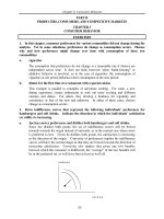
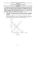
c. Draw a graph to illustrate your answers.
Equilibrium price and quantity are found at the intersection of the demand and
supply curves. When the income level increases in part b, the demand curve will
shift up and to the right. The intersection of the new demand curve and the supply
curve is the new equilibrium point.
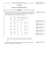
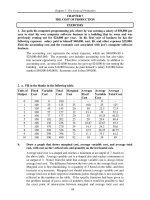
2. Consider a competitive market for which the quantities demanded and supplied (per
year) at various prices are given as follows:

Price
($)
Demand

(millions)
Supply
(millions)
60 22 14
80 20 16
100 18 18
120 16 20
a. Calculate the price elasticity of demand when the price is $80 and when the price is
$100.
We know that the price elasticity of demand may be calculated using equation 2.1
from the text:
Chapter 2: The Basics of Supply and Demand
E
Q
Q
P
P
P
Q
Q
P
D
D
D
D
D
==
Δ
Δ
Δ

Δ
.

With each price increase of $20, the quantity demanded decreases by 2.
Therefore,
ΔQ
D
ΔP
⎛
⎝
⎞
⎠
=
−2
20
=−0.1.

At P = 80, quantity demanded equals 20 and
E
D
=
80
20
⎛
⎝
⎞
⎠
−0.1
()
=−0.40.

Similarly, at P = 100, quantity demanded equals 18 and
E
D
=
100
18
⎛
⎝
⎞
⎠
−0.1
()
=−0.56.

b. Calculate the price elasticity of supply when the price is $80 and when the price is
$100.
The elasticity of supply is given by:
E
Q
Q
P
P
P
Q
Q
P
S
S
S

S
S
==
Δ
Δ
Δ
Δ
.

With each price increase of $20, quantity supplied increases by 2. Therefore,
ΔQ
S
ΔP
⎛
⎝
⎞
⎠
=
2
20
= 0.1.

At P = 80, quantity supplied equals 16 and
E
S
=
80
16
⎛
⎝

⎞
⎠
0.1
()
= 0.5.

Similarly, at P = 100, quantity supplied equals 18 and
E
S
=
100
18
⎛
⎝
⎞
⎠
0.1
()
= 0.56.

c. What are the equilibrium price and quantity?
The equilibrium price and quantity are found where the quantity supplied equals the
quantity demanded at the same price. As we see from the table, the equilibrium
price is $100 and the equilibrium quantity is 18 million.
d. Suppose the government sets a price ceiling of $80. Will there be a shortage, and if
so, how large will it be?
With a price ceiling of $80, consumers would like to buy 20 million, but producers
will supply only 16 million. This will result in a shortage of 4 million.
6

Chapter 2: The Basics of Supply and Demand
3. Refer to Example 2.5 on the market for wheat. At the end of 1998, both Brazil and
Indonesia opened their wheat markets to U.S. farmers. Suppose that these new markets add
200 million bushels to U.S. wheat demand. What will be the free market price of wheat and
what quantity will be produced and sold by U.S. farmers in this case?
The following equations describe the market for wheat in 1998:
Q
S
= 1944 + 207P
and
Q
D
= 3244 - 283P.
If Brazil and Indonesia add an additional 200 million bushels of wheat to U.S.
wheat demand, the new demand curve would be equal to Q
D
+ 200, or
Q
D
= (3244 - 283P) + 200 = 3444 - 283P.
Equating supply and the new demand, we may determine the new equilibrium price,
1944 + 207P = 3444 - 283P, or
490P = 1500, or P* = $3.06122 per bushel.
To find the equilibrium quantity, substitute the price into either the supply or
demand equation, e.g.,
Q
S
= 1944 + (207)(3.06122) = 2,577.67
and
Q

D
= 3444 - (283)(3.06122) = 2,577.67
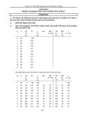
4. A vegetable fiber is traded in a competitive world market, and the world price is $9 per
pound. Unlimited quantities are available for import into the United States at this price.
The U.S. domestic supply and demand for various price levels are shown below.
Price U.S. Supply U.S. Demand
(million lbs.) (million lbs.)
3 2 34
6 4 28
9 6 22
12 8 16
15 10 10
18 12 4

a. What is the equation for demand? What is the equation for supply?
The equation for demand is of the form Q=a-bP. First find the slope, which is
ΔQ
Δ
P
=
−6
3
=−2 =−b.
You can figure this out by noticing that every time price
increases by 3, quantity demanded falls by 6 million pounds. Demand is now
Q=a-2P. To find a, plug in any of the price quantity demanded points from the table:
Q=34=a-2*3 so that a=40 and demand is Q=40-2P.
7

Chapter 2: The Basics of Supply and Demand

The equation for supply is of the form Q = c + dP. First find the slope, which is
ΔQ
Δ
P
=
2
3
= d.
You can figure this out by noticing that every time price increases
by 3, quantity supplied increases by 2 million pounds. Supply is now
Q = c +
2
3
P.
To find c plug in any of the price quantity supplied points from the
table:
Q = 2 = c +
2
3
(3)
so that c=0 and supply is
Q =
2
3
P.

b. At a price of $9, what is the price elasticity of demand? What is it at price of $12?
Elasticity of demand at P=9 is
P
Q

ΔQ
ΔP
=
9
22
(−2) =
−18
22
=−0.82.

Elasticity of demand at P=12 is
P
Q
ΔQ
ΔP
=
12
16
(−2) =
−24
16
=−1.5.

c. What is the price elasticity of supply at $9? At $12?
Elasticity of supply at P=9 is
P
Q
ΔQ
ΔP
=

9
6
2
3
⎛
⎝
⎞
⎠
=
18
18
=1.0.

Elasticity of supply at P=12 is
P
Q
ΔQ
ΔP
=
12
8
2
3
⎛
⎝
⎞
⎠
=
24
24

= 1.0.

d. In a free market, what will be the U.S. price and level of fiber imports?
With no restrictions on trade, world price will be the price in the United States, so
that P=$9. At this price, the domestic supply is 6 million lbs., while the domestic
demand is 22 million lbs. Imports make up the difference and are 16 million lbs.

5. Much of the demand for U.S. agricultural output has come from other countries. In
1998, the total demand for wheat was Q = 3244 - 283P. Of this, domestic demand was Q
D
=
1700 - 107P. Domestic supply was Q
S
= 1944 + 207P. Suppose the export demand for
wheat falls by 40 percent.

a. U.S. farmers are concerned about this drop in export demand. What happens to the
free market price of wheat in the United States? Do the farmers have much reason
to worry?

Given total demand, Q = 3244 - 283P, and domestic demand, Q
d
= 1700 - 107P, we
may subtract and determine export demand, Q
e
= 1544 - 176P.
The initial market equilibrium price is found by setting total demand equal to
supply:
3244 - 283P = 1944 + 207P, or
P = $2.65.

The best way to handle the 40 percent drop in export demand is to assume that the
export demand curve pivots down and to the left around the vertical intercept so that
at all prices demand decreases by 40 percent, and the reservation price (the
maximum price that the foreign country is willing to pay) does not change. If you
8

Chapter 2: The Basics of Supply and Demand
instead shifted the demand curve down to the left in a parallel fashion the effect on
price and quantity will be qualitatively the same, but will differ quantitatively.
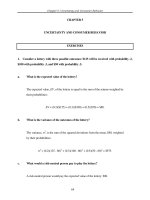
The new export demand is 0.6Q
e
=0.6(1544-176P)=926.4-105.6P. Graphically,
export demand has pivoted inwards as illustrated in figure 2.5a below.
Total demand becomes
Q
D
= Q
d
+ 0.6Q
e
= 1700 - 107P + 926.4-105.6P = 2626.4 - 212.6P.

Q
e
1544
926.4
8.77
P

Figure 2.5a

Equating total supply and total demand,
1944 + 207
P
= 2626.4 - 212.6
P
, or
P
= $1.63,
which is a significant drop from the market-clearing price of $2.65 per bushel. At
this price, the market-clearing quantity is 2280.65 million bushels. Total revenue
has decreased from $6614.6 million to $3709.0 million. Most farmers would
worry.
b. Now suppose the U.S. government wants to buy enough wheat each year to raise the
price to $3.50 per bushel. With this drop in export demand, how much wheat would
the government have to buy? How much would this cost the government?

With a price of $3.50, the market is not in equilibrium. Quantity demanded and
supplied are
Q
D
= 2626.4-212.6(3.5)=1882.3, and
Q
S
= 1944 + 207(3.5) = 2668.5.
Excess supply is therefore 2668.5-1882.3=786.2 million bushels. The government
must purchase this amount to support a price of $3.5, and will spend
$3.5(786.2 million) = $2751.7 million per year.
6. The rent control agency of New York City has found that aggregate demand is
9