Tài liệu Bài tập về Kinh tế vĩ mô bằng tiếng Anh - Chương 4: Cá nhân và nhu cầu thị trường doc

Chapter 4: Individual and Market Demand

41
CHAPTER 4
INDIVIDUAL AND MARKET DEMAND
EXERCISES

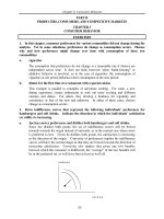
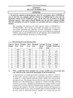
1. An individual sets aside a certain amount of his income per month to spend on his two hobbies, collecting
wine and collecting books. Given the information below, illustrate both the price consumption curve
associated with changes in the price of wine, and the demand curve for wine.
Price
Wine
Price
Book
Quantity
Wine
Quantity
Book
Budget
$10 $10 7 8 $150
$12 $10 5 9 $150
$15 $10 4 9 $150
$20 $10 2 11 $150

The price consumption curve connects each of the four optimal bundles given in the table above.
As the price of wine increases, the budget line will pivot inwards and the optimal bundle will
change.
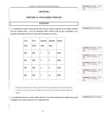
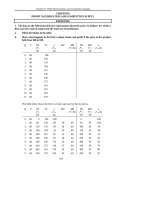
2. An individual consumes two goods, clothing and food. Given the information below, illustrate the income
consumption curve, and the Engel curves for clothing and food.

Formatted: Space Before: 1.2 line,

After: 1.2 line, Line spacing: 1.5
lines
Formatted: Bullets and Numbering
Formatted: Space Before: 1.2 line,
After: 1.2 line, Line spacing: 1.5
lines
Formatted: Space Before: 1.2 line,
After: 1.2 line, Line spacing: 1.5
lines
Formatted: Space Before: 1.2 line,
After: 1.2 line, Line spacing: 1.5
lines
Formatted: Space Before: 1.2 line,
After: 1.2 line, Line spacing: 1.5
lines
Formatted: Space Before: 1.2 line,
After: 1.2 line, Line spacing: 1.5
lines
Formatted: Bullets and Numbering
Chapter 4: Individual and Market Demand

42
Price
Clothing
Price
Food
Quantity
Clothing
Quantity
Food

Income
$10 $2 6 20 $100
$10 $2 8 35 $150
$10 $2 11 45 $200
$10 $2 15 50 $250

The income consumption curve connects each of the four optimal bundles given in the table
above. As the individual’s income increases, the budget line will shift out and the optimal bundle
will change. The Engel curves for each good illustrate the relationship between the quantity
consumed and income (on the vertical axis). Both Engel curves are upward sloping.

C
F
income consumption curve

Formatted: Space Before: 1.2 line,
After: 1.2 line, Line spacing: 1.5
lines
Formatted: Space Before: 1.2 line,
After: 1.2 line, Line spacing: 1.5
lines
Formatted: Space Before: 1.2 line,
After: 1.2 line, Line spacing: 1.5
lines
Formatted: Space Before: 1.2 line,
After: 1.2 line, Line spacing: 1.5
lines
Formatted: Space Before: 1.2 line,
After: 1.2 line, Line spacing: 1.5
lines

Chapter 4: Individual and Market Demand

43
I
F

I
C

3. Jane always gets twice as much utility from an extra ballet ticket as she does from an extra basketball
ticket, regardless of how many tickets of either type she has. Draw Jane’s income consumption curve and her
Engel curve for ballet tickets.
Jane will consume either all ballet tickets or all basketball tickets, depending on the two prices.
As long as ballet tickets are less than twice the price of basketball tickets, she will choose all
ballet. If ballet tickets are more than twice the price of basketball tickets then she will choose all
basketball. This can be determined by comparing the marginal utility per dollar for each type of
ticket, where her marginal utility of another ballet ticket is 2 and her marginal utility of another
basketball ticket is 1. Her income consumption curve will then lie along the axis of the good that
she chooses. As income increases, and the budget line shifts out, she will stick with the chosen
good. The Engel curve is a linear, upward-sloping line. For any given increase in income, she
will be able to purchase a fixed amount of extra tickets.

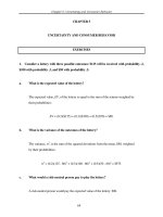
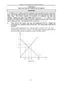
4. a. Orange juice and apple juice are known to be perfect substitutes. Draw the appropriate price-
consumption (for a variable price of orange juice) and income-consumption curves.
We know that the indifference curves for perfect substitutes will be straight lines. In this case, the
consumer will always purchase the cheaper of the two goods. If the price of orange juice is less than
Formatted: Bullets and Numbering
Chapter 4: Individual and Market Demand

44

that of apple juice, the consumer will purchase only orange juice and the price consumption curve
will be on the “orange juice axis” of the graph (point F). If apple juice is cheaper, the consumer will
purchase only apple juice and the price consumption curve will be on the “apple juice axis” (point
E). If the two goods have the same price, the consumer will be indifferent between the two; the price
consumption curve will coincide with the indifference curve (between E and F). See the figure
below.
Apple J uice
Orange Juice
U
E
F
P
A
= P
O
P
A
> P
O
P
A
< P
O

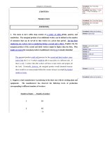
Assuming that the price of orange juice is less than the price of apple juice, the consumer will
maximize her utility by consuming only orange juice. As the level of income varies, only the
amount of orange juice varies. Thus, the income consumption curve will be the “orange juice axis”
in the figure below.
Chapter 4: Individual and Market Demand

45
Apple J uice
Orange Juice
U
2
U
1
U
3
Budget
Constraint
Income
Consumption
Curve

4.b. Left shoes and right shoes are perfect complements. Draw the appropriate price-consumption and income-
consumption curves.
For goods that are perfect complements, such as right shoes and left shoes, we know that the
indifference curves are L-shaped. The point of utility maximization occurs when the budget
constraints, L
1
and L
2
touch the kink of U
1
and U
2
. See the following figure.
Left Shoes
U

2
U
1
Right
Shoes
L
1
L
2
Price
Consumption
Curve

In the case of perfect complements, the income consumption curve is also a line through the corners
of the L-shaped indifference curves. See the figure below.
Chapter 4: Individual and Market Demand

46
Left Shoes
U
2
U
1
Right
Shoes
L
1
L
2
Income

Consumption
Curve

5. Each week, Bill, Mary, and Jane select the quantity of two goods,
x
1
and x
2
, that they will consume in
order to maximize their respective utilities. They each spend their entire weekly income on these two goods.
a. Suppose you are given the following information about the choices that Bill makes over a three-
week
period:


x
1

x
2

P
1

P
2

I
Week 1 10 20 2 1 40
Week 2 7 19 3 1 40

Week 3 8 31 3 1 55

Did Bill’s utility increase or decrease between week 1 and week 2? Between week 1 and week 3?
Explain using a graph to support your answer.
Formatted: Bullets and Numbering
Formatted: Space Before: 1.2 line,
After: 1.2 line, Line spacing: 1.5
lines
Formatted: Space Before: 1.2 line,
After: 1.2 line, Line spacing: 1.5
lines
Formatted: Space Before: 1.2 line,
After: 1.2 line, Line spacing: 1.5
lines
Formatted: Space Before: 1.2 line,
After: 1.2 line, Line spacing: 1.5
lines
Deleted:
Deleted: How about between
Chapter 4: Individual and Market Demand

47
Bill’s utility fell between weeks 1 and 2 since he ended up with less of both goods. In week 2, the
price of good 1 rose and his income remained constant. The budget line will pivot inwards and he
will have to move to a lower indifference curve. Between week 1 and week 3 his utility rose. The
increase in income more than compensated him for the rise in the price of good 1. Since the price
of good 1 rose by $1, he would need an extra $10 to afford the same bundle of goods that he chose
in week 1. This can be found by multiplying week 1 quantities times week 2 prices. However, his
income went up by $15, so his budget line shifted out beyond his week 1 bundle. Therefore, his
original bundle lies within his new budget set, and his new week 3 bundle is on a higher

indifference curve.
b. Now consider the following information about the choices that Mary makes:


x
1

x
2

P
1

P
2

I
Week 1 10 20 2 1 40
Week 2 6 14 2 2 40
Week 3 20 10 2 2 60

Did Mary’s utility increase or decrease between week 1 and week 3? Does Mary consider both goods
to be normal goods? Explain.
Mary’s utility went up. To afford the week 1 bundle at the new prices, she would need an extra
$20, which is exactly what happened to her income. However, since she could have chosen the
original bundle at the new prices and income but chose not to, she must have found a bundle that
left her slightly better off. In the graph below, the week 1 bundle is at the intersection of the week
1 and week 3 budget lines. The week 3 bundle is somewhere on the line segment that lies above
the week 1 indifference curve. This bundle will be on a higher indifference curve. A good is
normal if more is chosen when income increases. Good 2 is not normal because when her income

went up from week 2 to week 3, she consumed less of the good (holding prices the same).
Formatted: Space Before: 1.2 line,
After: 1.2 line, Line spacing: 1.5
lines
Formatted: Space Before: 1.2 line,
After: 1.2 line, Line spacing: 1.5
lines
Formatted: Space Before: 1.2 line,
After: 1.2 line, Line spacing: 1.5
lines
Formatted: Space Before: 1.2 line,
After: 1.2 line, Line spacing: 1.5
lines