Tài liệu Bài tập về Kinh tế vĩ mô bằng tiếng Anh - Chương 9 pptx

Chapter 9: The Analysis of Competitive Markets

117
CHAPTER 9
THE ANALYSIS OF COMPETITIVE MARKETS
EXERCISES
1. In 1996, the U.S. Congress raised the minimum wage from $4.25 per hour to $5.15 per
hour. Some people suggested that a government subsidy could help employers finance the
higher wage. This exercise examines the economics of a minimum wage and wage
subsidies. Suppose the supply of low-skilled labor is given by
L w
S
=10
, where L
S
is the
quantity of low-skilled labor (in millions of persons employed each year) and w is the wage
rate (in dollars per hour). The demand for labor is given by
L w
D
=80 -10
.
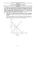
a. What will the free market wage rate and employment level be? Suppose the
government sets a minimum wage of $5 per hour. How many people would then be
employed?
In a free-market equilibrium, L
S
= L
D
. Solving yields w = $4 and L
S

= L
D
= 40. If the
minimum wage is $5, then L
S
= 50 and L
D
= 30. The number of people employed will be
given by the labor demand, so employers will hire 30 million workers.
L
S
L
D
30
40 50
8
5
4
80
L
W

Figure 9.1.a
Chapter 9: The Analysis of Competitive Markets

118
b. Suppose that instead of a minimum wage, the government pays a subsidy of $1 per
hour for each employee. What will the total level of employment be now? What
will the equilibrium wage rate be?
Let w denote the wage received by the employee. Then the employer receiving

the $1 subsidy per worker hour only pays w-1 for each worker hour. As shown in
Figure 9.1.b, the labor demand curve shifts to:
L
D
= 80 - 10 (w-1) = 90 - 10w,
where w represents the wage received by the employee.
The new equilibrium will be given by the intersection of the old supply curve with
the new demand curve, and therefore, 90-10
W
** = 10
W
**, or w** = $4.5 per hour
and L** = 10(4.5) = 45 million persons employed. The real cost to the employer
is $3.5 per hour.
W
L = 10w
s
9
8
4.5
4
40
45
80
90
wage and employment
after subsidy
L = 90-10w
D
(subsidy)

L = 80-10w
D
L
Figure 9.1.b

2. Suppose the market for widgets can be described by the following equations:
Demand: P = 10 - Q Supply: P = Q - 4
where P is the price in dollars per unit and Q is the quantity in thousands of units.

a. What is the equilibrium price and quantity?

To find the equilibrium price and quantity, equate supply and demand and solve for
Q
EQ
:
10 -
Q
=
Q
- 4, or
Q
EQ

= 7.

Substitute
Q
EQ
into either the demand equation or the supply equation to obtain
P

EQ
.

P
EQ
= 10 - 7 = 3,
or
P
EQ
= 7 - 4 = 3.
b. Suppose the government imposes a tax of $1 per unit to reduce widget consumption
and raise government revenues. What will the new equilibrium quantity be? What
price will the buyer pay? What amount per unit will the seller receive?

Chapter 9: The Analysis of Competitive Markets

119
With the imposition of a $1.00 tax per unit, the demand curve for widgets shifts
inward. At each price, the consumer wishes to buy less. Algebraically, the new
demand function is:
P
= 9 -
Q
.


The new equilibrium quantity is found in the same way as in (2a):
9 -
Q
=

Q
- 4, or
Q
* = 6.5.
To determine the price the buyer pays,
P
B
*
, substitute
Q
* into the demand equation:
P
B
*
= 10 - 6.5 = $3.50.
To determine the price the seller receives,
P
S
*
, substitute
Q
* into the supply
equation:
P
S
*
= 6.5 - 4 = $2.50.
c. Suppose the government has a change of heart about the importance of widgets to the
happiness of the American public. The tax is removed and a subsidy of $1 per unit is
granted to widget producers. What will the equilibrium quantity be? What price will

the buyer pay? What amount per unit (including the subsidy) will the seller receive?
What will be the total cost to the government?

The original supply curve for widgets was
P
=
Q
- 4. With a subsidy of $1.00 to
widget producers, the supply curve for widgets shifts outward. Remember that the
supply curve for a firm is its marginal cost curve. With a subsidy, the marginal cost
curve shifts down by the amount of the subsidy. The new supply function is:
P
=
Q
- 5.
To obtain the new equilibrium quantity, set the new supply curve equal to the
demand curve:
Q
- 5 = 10 -
Q
, or
Q
= 7.5.
The buyer pays
P
= $2.50, and the seller receives that price plus the subsidy, i.e.,
$3.50. With quantity of 7,500 and a subsidy of $1.00, the total cost of the subsidy to
the government will be $7,500.

3. Japanese rice producers have extremely high production costs, in part due to the high

opportunity cost of land and to their inability to take advantage of economies of large-scale
production. Analyze two policies intended to maintain Japanese rice production: (1) a per-
pound subsidy to farmers for each pound of rice produced, or (2) a per-pound tariff on
imported rice. Illustrate with supply-and-demand diagrams the equilibrium price and
quantity, domestic rice production, government revenue or deficit, and deadweight loss from
each policy. Which policy is the Japanese government likely to prefer? Which policy are
Japanese farmers likely to prefer?

Figure 9.3.a shows the gains and losses from a per-pound subsidy with domestic
supply,
S
, and domestic demand,
D
.
P
S
is the subsidized price,
P
B
is the price paid
by the buyers, and
P
EQ
is the equilibrium price without the subsidy, assuming no
imports. With the subsidy, buyers demand
Q
1
. Farmers gain amounts equivalent to
Chapter 9: The Analysis of Competitive Markets

120
areas
A
and
B
. This is the increase in producer surplus. Consumers gain areas
C

and
F
. This is the increase in consumer surplus. Deadweight loss is equal to the
area
E
. The government pays a subsidy equal to areas
A + B + C + F + E
.

Figure 9.3.b shows the gains and losses from a per-pound tariff.
P
W
is the world
price, and
P
EQ
is the equilibrium price. With the tariff, assumed to be equal to
P
EQ
-

P

W
, buyers demand
Q
T
, farmers supply
Q
D
, and
Q
T
-
Q
D
is imported. Farmers gain
a surplus equivalent to area
A
. Consumers lose areas
A, B, C
; this is the decrease in
consumer surplus. Deadweight loss is equal to the areas
B
and
C
.

Price
Quantity
S
D
P

B
P
EQ
P
S
A
C
B
E
F
Q
EQ
Q
1

Figure 9.3.a
Price
S
D
P
EQ
P
W
A
C
B
Q
EQ
Q
T

Q
D
Quantity

Figure 9.3.b
Without more information regarding the size of the subsidy and the tariff, and the
specific equations for supply and demand, it seems sensible to assume that the
Chapter 9: The Analysis of Competitive Markets

121
Japanese government would avoid paying subsidies by choosing a tariff, but the
rice farmers would prefer the subsidy.
4. In 1983, the Reagan Administration introduced a new agricultural program called the
Payment-in-Kind Program. To see how the program worked, let’s consider the wheat
market.
a. Suppose the demand function is Q
D
= 28 - 2P and the supply function is Q
S
= 4 + 4P,
where P is the price of wheat in dollars per bushel and Q is the quantity in billions of
bushels. Find the free-market equilibrium price and quantity.

Equating demand and supply,
Q
D
= Q
S
,
28 - 2

P
= 4 + 4
P
, or
P
= 4.

To determine the equilibrium quantity, substitute
P
= 4 into either the supply
equation or the demand equation:
Q
S
= 4 + 4(4) = 20
and
Q
D
= 28 - 2(4)

= 20.
b. Now suppose the government wants to lower the supply of wheat by 25 percent from
the free-market equilibrium by paying farmers to withdraw land from production.
However, the payment is made in wheat rather than in dollars--hence the name of the
program. The wheat comes from the government’s vast reserves that resulted from
previous price-support programs. The amount of wheat paid is equal to the amount
that could have been harvested on the land withdrawn from production. Farmers are
free to sell this wheat on the market. How much is now produced by farmers? How
much is indirectly supplied to the market by the government? What is the new
market price? How much do the farmers gain? Do consumers gain or lose?

Because the free market supply by farmers is 20 billion bushels, the 25 percent
reduction required by the new Payment-In-Kind (PIK) Program would imply that
the farmers now produce 15 billion bushels. To encourage farmers to withdraw
their land from cultivation, the government must give them 5 billion bushels, which
they sell on the market.
Because the total supply to the market is still 20 billion bushels, the market price
does not change; it remains at $4 per bushel. The farmers gain $20 billion, equal to
($4)(5 billion bushels), from the PIK Program, because they incur no costs in
supplying the wheat (which they received from the government) to the market. The
PIK program does not affect consumers in the wheat market, because they purchase
the same amount at the same price as they did in the free market case.
c. Had the government not given the wheat back to the farmers, it would have stored or
destroyed it. Do taxpayers gain from the program? What potential problems does
the program create?

Taxpayers gain because the government is not required to store the wheat.
Although everyone seems to gain from the PIK program, it can only last while there
are government wheat reserves. The PIK program assumes that the land removed
from production may be restored to production when stockpiles are exhausted. If
this cannot be done, consumers may eventually pay more for wheat-based products.
Chapter 9: The Analysis of Competitive Markets

122
5.

About 100 million pounds of jelly beans are consumed in the United States each year, and
the price has been about 50 cents per pound. However, jelly bean producers feel that their
incomes are too low, and they have convinced the government that price supports are in
order. The government will therefore buy up as many jelly beans as necessary to keep the
price at $1 per pound. However, government economists are worried about the impact of

this program, because they have no estimates of the elasticities of jelly bean demand or
supply.

a. Could this program cost the government more than $50 million per year? Under
what conditions? Could it cost less than $50 million per year? Under what
conditions? Illustrate with a diagram.

If the quantities demanded and supplied are very responsive to price changes, then a
government program that doubles the price of jelly beans could easily cost more
than $50 million. In this case, the change in price will cause a large change in
quantity supplied, and a large change in quantity demanded. In Figure 9.5.a.i, the
cost of the program is (Q
S
-Q
D
)*$1. Given Q
S
-Q
D
is larger than 50 million, then the
government will pay more than 50 million dollars. If instead supply and demand
were relatively price inelastic, then the change in price would result in very small
changes in quantity supplied and quantity demanded and (Q
S
-Q
D
) would be less
than $50 million, as illustrated in figure 9.5.a.ii.
b. Could this program cost consumers (in terms of lost consumer surplus) more than $50
million per year? Under what conditions? Could it cost consumers less than $50

million per year? Under what conditions? Again, use a diagram to illustrate.

When the demand curve is perfectly inelastic, the loss in consumer surplus is $50
million, equal to ($0.5)(100 million pounds). This represents the highest possible
loss in consumer surplus. If the demand curve has any elasticity at all, the loss in
consumer surplus would be less then $50 million. In Figure 9.5.b, the loss in
consumer surplus is area A plus area B if the demand curve is D and only area A if
the demand curve is D’.
Q
P
Q
S
Q
D
1.00
.50
100
D
S

Chapter 9: The Analysis of Competitive Markets

123
Figure 9.5.a.i

Q
P
Q
S
Q

D
1.00
.50
100
D
S

Figure 9.5.a.ii

Q
P
D’
D
S
A
B
100
1.00
.50

Figure 9.5.b
Chapter 9: The Analysis of Competitive Markets

124
6. In Exercise 4 of Chapter 2, we examined a vegetable fiber traded in a competitive world
market and imported into the United States at a world price of $9 per pound. U.S. domestic
supply and demand for various price levels are shown in the following table.
Price U.S. Supply
(million pounds)
U.S. Demand

(million pounds)
3 2 34
6 4 28
9 6 22
12 8 16
15 10 10
18 12 4
Answer the following about the U.S. market:
a. Confirm that the demand curve is given by
Q
D
= 40 − 2P
, and that the supply curve is
given by
Q
S
=
2
3
P
.

To find the equation for demand, we need to find a linear function Q
D
= a + bP
such that the line it represents passes through two of the points in the table such as
(15,10) and (12,16). First, the slope, b, is equal to the “rise” divided by the “run,”
ΔQ
Δ
P

=
10
−16
15
−12
=−2 = b.

Second, we substitute for b and one point, e.g., (15, 10), into our linear function to
solve for the constant, a:
10 = a − 215
( )
, or a = 40.
Therefore,
Q
D
= 40 − 2P.

Similarly, we may solve for the supply equation Q
S
= c + dP passing through two
points such as (6,4) and (3,2). The slope, d, is

ΔQ
Δ
P
=
4
− 2
6
− 3

=
2
3
.
.
Solving for c:
4 = c +
2
3
⎛
⎝
⎞
⎠
6
()
, or c = 0.
Therefore,
Q
S
=
2
3
⎛
⎝
⎞
⎠
P.

b. Confirm that if there were no restrictions on trade, the U.S. would import 16 million
pounds.

If there are no trade restrictions, the world price of $9.00 will prevail in the U.S.
From the table, we see that at $9.00 domestic supply will be 6 million pounds.
Similarly, domestic demand will be 22 million pounds. Imports will provide the
difference between domestic demand and domestic supply: 22 - 6 = 16 million
pounds.