Tài liệu Adaptive WCDMA (P3) pdf
Bạn đang xem bản rút gọn của tài liệu. Xem và tải ngay bản đầy đủ của tài liệu tại đây (357.87 KB, 35 trang )
3
Code acquisition
3.1 OPTIMUM SOLUTION
In this case, the theory starts with a simple problem where, for a received signal r(t) =
s(t, θ) + n(t), we have to estimate a generalized time invariant vector of parameters θ
(frequency, phase, delay, data, ...) of a signal s(t, θ) in the presence of Gaussian noise
n(t). The best that we can do is to find an estimate
ˆ
θ of the parameter θ for which
the aposterior probability p(
ˆ
θ/r) is maximum; hence the name maximum aposterior
probability (MAP) estimate. In other words, the chosen estimate based on the received
signal r is correct for the highest probability. Practical implementation requires us to
locally generate a number of trial values
˜
θ,toevaluatep(
˜
θ/r) for each such value and
then to choose
˜
θ =
ˆ
θ for which p(
˜
θ/r) is maximum. In this chapter, we focus only on
code acquisition and parameter θ will include only code delay θ ={τ } and become a
scalar. Analytically, this can be expressed as
MAP ⇒
ˆ
θ = arg max p(
˜
θ/r) (3.1)
Very often, in practice, evaluation of p(
˜
θ/r) in closed form is not possible. By using the
Bayesian rule for the joint probability distribution function
p(r,
˜
θ) = p(r)p(
˜
θ/r) = p(
˜
θ)p(r/
˜
θ) (3.2)
and assuming a uniform prior distribution of θ, maximizing p(
˜
θ/r) becomes equivalent
to maximizing p(r/
˜
θ), a function that can be determined more easily. This algorithm is
known as maximum likelihood (ML) estimation and can be defined analytically as
ML ⇒
ˆ
θ = arg max p(r/
˜
θ) (3.3)
It is straightforward to show that in the case of Gaussian noise, the ML principle necessi-
tates the search for that value of θ that would maximize the likelihood function defined as
λ(
˜
θ) =
r(t)s(t,
˜
θ)dt −
s
2
(t,
˜
θ)dt(3.4)
Adaptive WCDMA: Theory And Practice.
Savo G. Glisic
Copyright
2003 John Wiley & Sons, Ltd.
ISBN: 0-470-84825-1
44
CODE ACQUISITION
where s(t,
˜
θ) is the locally generated replica of the signal with a trial value
˜
θ.For
the given signal power, the second term in the previous equation is a constant so that
the maximization is equivalent to the maximization of the first term only. This can be
expressed as
λ(
˜
θ) =
r(t)s(t,
˜
θ)dt(3.5)
Instead of searching for the maximum of λ(
˜
θ) in a so-called open loop configuration, an
equivalent procedure would be to find the zero of the first derivative of λ(
˜
θ)
MLT ⇒
ˆ
θ = arg zero
∂λ(
˜
θ)
∂
˜
θ
= arg zero
r(t)
∂s(t,
˜
θ)
∂
˜
θ
dt
(3.6)
This structure is known as the maximum likelihood tracker (MLT). In practice, the signal
derivative is often approximated by the signal difference
∂s(t,
˜
θ)
∂
˜
θ
=
1
2θ
{s(t,
˜
θ + θ ) − s(t,
˜
θ − θ)} (3.7)
where s(t,
˜
θ + θ ) and s(t,
˜
θ − θ ) are so called early and late versions of the local
signal with respect to the generalized parameter θ to be estimated. This results in the
so-called early–late tracker
ELT ⇒
ˆ
θ = arg zero{E(t,
˜
θ) − L(t,
˜
θ)} (3.8)
where
E(t,
˜
θ) =
1
2θ
r(t)s(t,
˜
θ + θ )dt
L(t,
˜
θ) =
1
2θ
r(t)s(t,
˜
θ − θ )dt
(3.9)
In the case of code synchronization, θ = τ and the ML synchronizing receiver implied by
equation (3.5) should, in principle, create all possible time-offset versions of the known
code waveform, correlate all of them with the received data and choose the ˜τ corre-
sponding to the largest correlation as its estimate, ˆτ
ML
. Owing to the continuous range
of values of τ , this is not possible in practice and some type of range quantization is
necessary. The resulting candidate values are called cells, and the initial parameter esti-
mation problem is translated into a multiple-hypothesis problem: to locate the cell most
likely to contain the unknown offset, given this piece of data. This is exactly the coarse
code synchronization or code acquisition problem, the result of which is to resolve the
code phase (or the ‘epoch’) ambiguity within the size of the cell. Since this remaining
error is typically larger than desired, further operations are required in order to reduce
it to acceptable levels. This remaining part of the synchronization task, namely, that of
PRACTICAL SOLUTIONS
45
fine synchronization or code tracking, is performed by one of the available code-tracking
loops, which we discuss in the next chapter.
Once the nature and size of these cells have been determined, the next question is how
to go about performing the search most successfully. Clearly, the strategy will depend on a
variety of factors such as criteria of performance, degree of complexity and computational
power available (directly related to cost), prior available information about the location of
the correct cell and so on. A brute-force approach would try to create a bank of parallel
correlation branches, each matched to a possible quantized value of the timing offset;
it would then process the received waveform through all of them simultaneously, pick
the largest and declare a candidate solution. Unless the uncertainty region (number of
cells) is small, corresponding to either a small code period or a small initial uncertainty,
such a solution (which we may call the totally parallel solution) becomes obviously
unwieldy in complexity very quickly. We note, however, that small uncertainty regions
may be encountered in a nested design, whereby a multitude of different-period codes are
combined for precisely the purpose of aiding acquisition. Furthermore, neural network
structures are currently being explored for this purpose, where the neural network is
trained for all possible such values. Such a scheme would emulate the spirit (if not the
exact statistical processing) of the above solutions.
3.2 PRACTICAL SOLUTIONS
In practice, most of the time total parallelism is out of the question when the number
of cells is very large (although it appears doable for smaller uncertainty regions) and
simpler solutions are necessary. One of the most familiar of such approaches is the
simple technique of serial search, where the search starts from a specific cell and serially
examines the remaining cells in some direction and in a prespecified order until the
correct cell is found. Hence, serial search techniques do not account for any additional
information gathered during the past search time, which could conceivably be used to
alter the direction of search toward cells that show increased posterior likelihood of being
the correct ones. A serial search starts from a cell that could be chosen totally arbitrarily
(no prior information), or by some prior knowledge about a likely cell, and proceeds
in a simple and easily implementable predirected manner. When the uncertainty space
(collection of all possible cells) is two-dimensional (delay and frequency offset) and
searching all possible cells serially appears to be very time consuming, a speedup may
be achieved by employing a bank of filters, each matched to a possible Doppler offset.
The same idea can be applied to the one-dimensional case (no frequency uncertainty),
where now a bank of correlators may be employed, each starting from a different point of
the uncertainty region. This effectively amounts to dividing the search in many parallel
subsearches and therefore reducing the total search time by a proportional amount.
One should be aware that although it holds true that only one cell contains the exact
delay and Doppler offsets of the incoming code, the set of desirable cells acceptable to
the receiver includes a number of cells adjacent to the exact one. Indeed, the receiver will
terminate acquisition and initiate tracking, the first time a cell is reached (and correctly
identified), which is close enough to true synchronization so that the tracking loop can pull
46
CODE ACQUISITION
in and perform the remaining synchronization operation successfully. All these desirable
cells are collectively called hypothesis H
1
, and the remaining nondesirable ‘out-of-sync’
cells comprise hypothesis H
0
. As an example, consider the case in which the receiver
examines the code delay uncertainty in steps of half a chip time (δt = T
c
/2) and there
is no frequency uncertainty. Then, all four cells located in the interval (−T
c
,T
c
) around
the true delay of the incoming code are included in hypothesis H
1
, since some amount
of code correlation exists for each one of these cells, an amount that can initiate the
code-tracking loop.
The above definition of cells and hypotheses implies that each test does not pertain
to a single value of the unknown parameter τ , but rather to a range of values. It is
straightforward to show that, under mild conditions and approximations pertaining to the
pseudorandom nature of the code, this reformulated hypothesis testing results in a statistic
(correlation) and threshold setting that do not depend on the given (tested) value of the
unknown parameter (a uniformly most powerful test). This is because the threshold value
is set by the desirable probability of false alarm per cell (see below), which is independent
of τ under H
0
.
To recapitulate, the two-dimensional time/frequency code offset uncertainty within the
noisy received waveform is quantized into a number of cells, which are typically searched
in a serial fashion by a correlation receiver, although parallel multiple branches are also
possible. Motivated by an ML argument, the receiver creates a cross-correlation between
the incoming waveform and the local code at a specific offset, whose output is used to
decide whether the currently examined cell is a desirable (H
1
) one. The process continues
until one such cell is correctly identified. At that point, acquisition is terminated and
tracking is initiated.
3.3 CODE ACQUISITION ANALYSIS
The serial code acquisition can be represented by using the signal flow graph theory. Each
cell is represented by a node of a graph and transitions between the nodes depend on the
outcome of the decision in a given cell. Branches connecting the nodes characterize these
transitions. To motivate the operation in a transform domain, let us consider the simple
model of a process represented by the graph in Figure 3.1 and evaluate the probability
p
ac
(t) that the process will move from a to c in exactly t seconds.
To do this, we will introduce an additional variable τ to designate the time needed for
the process to move from a to b, characterized by the probability p
ab
(τ ). The parameter
a
b
c
t
t
Figure 3.1 Signal flow graph for a 3-state process.
CODE ACQUISITION ANALYSIS
47
p
ac
(t, τ ) represents the joint probability that the process moves from a to c in t seconds
and takes τ seconds to move from a to b. This probability can be represented as
p
ac
(t, τ ) = p
ab
(τ )p
bc
(t − τ) (3.10)
resulting in
p
ac
(t) =
p
ac
(t, τ ) dτ =
p
ab
(τ )p
bc
(t − τ)dτ
= p
ac
(t)
∗
p
bc
(t) (3.11)
In other words, the overall probability p
ac
(t) is a convolution of the two intermode
transition probabilities p
ab
and p
bc
. It is clear that for the graph with a large number
of nodes we will have to deal with multiple convolutions giving rise to computational
complexity. In this case, people being involved in electrical engineering prefer to move to
a transform domain, either Laplace (s) domain for continuous variables or into z-domain
for desecrate variables. This leads to using z-transform for the decision process flow graph
representation and multiple convolutions will be now replaced with multiple products
making the calculus much simpler. If p
ij
(n) is the probability for the process to move
from node i to node j in exactly n steps, then its z-transform
P
i,j
(z) =
∞
n=0
z
n
p
ij
(n) (3.12)
is called the probability generating function. For the analysis to follow, we will need a
few relations derived from this definition. First of all, the first and the second derivative
of this function can be represented as
∂
∂z
P
ij
(z) =
∞
n=0
np
ij
(n)z
n−1
(3.13)
∂
2
∂z
2
P
ij
(z) =
∞
n=0
n(n − 1)p
ij
(n)z
n−2
(3.14)
By definition, the average number of steps to move from node i to node j is
n =
∞
n=0
np
ij
(n) =
∂
∂z
P
ij
(z)
z=1
(3.15)
and the average time to do it can be represented as
t
ij
= T
ij
= nT =
∂
∂z
P
ij
(z)
z=1
· T(3.16)
48
CODE ACQUISITION
where T is the cell observation time that is, the time needed to create the decision variable
that will be referred to as dwell time. For the variance, we start with the definition
σ
2
T
= (n
2
− n
2
)T
2
(3.17)
The second derivative of the generating function can be represented as
∂
2
∂z
2
P
ij
(z)
z=1
=
∞
n=0
n
2
p
ij
(n) −
∞
n=0
np
ij
(n) = n
2
− n(3.18)
By using equations (3.15) and (3.18) in equation (3.17), the variance of time t
ij
can be
expressed in the following form:
σ
2
T
=
∂
2
P
ij
(z)
∂z
2
+
∂P
ij
(z)
∂z
−
∂P
ij
(z)
∂z
2
z=1
T
2
(3.19)
In what follows, we will use these few relations to analyze serial search code acquisition.
In order to get an initial insight into this method, we will assume that there are q cells to
be searched. Parameter q may be equal to the length of the pseudonoise (PN) code to be
searched or some multiple of it. For example, if the update size is one-half chip, q will
be twice the code length to be searched. Further assume that if a ‘hit’ (output is above
threshold) is detected by the threshold detector, the system goes into a verification mode
that may include both, an extended duration dwell time and an entry into a code loop
tracking mode. In any event, we model the ‘penalty’ of obtaining a false alarm as Kτ
d
second and the dwell time itself as τ
d
second. If a true hit is observed, the system has
acquired the signal, and the search is completed. Assume that the false alarm probability
P
FA
and the probability of detection P
D
are given. We will also assume that only one cell
represents the synchro position. Let each cell be numbered from left to right so that the
kth cell has apriori probability of having the signal present, given that it was not present
in cells 1 through k − 1, of
p
k
=
1
q + 1 − k
(3.20)
The generating function flow diagram is given in Figure 3.2 using the rule that at each
node the sum of the probability emanating from the node equals unity. The unit time rep-
resents τ
d
seconds and Kτ
d
seconds are represented in z-transform by z
K
. Consider node
1. The apriori probability of having the signal present is P
1
= 1/q, and the probability
of it not being present in the cell is 1 − P
1
. Suppose the signal was not present. Then we
advance to the next node (node 1a); since it corresponds to a probabilistic decision and
not a unit time delay, no z multiplies the branch going to it. At node 1a a false alarm
may occur, with probability P
FA
= α. This would require one unit of time to decide (τ
d
s)
and then K units of time (Kτ
d
s) are needed in verification mode to determine that there
was a false alarm. False alarms will not occur with probability (1 − α). This would take
one dwell time to decide and is represented by (1 − α)z branch going to node 2.
CODE ACQUISITION ANALYSIS
49
F
S
P
D
Z
P
1
P
FA3
Z
k
+1
P
FA1
Z
k
+1
P
FAq
Z
k
+1
P
FA2
Z
k +1
(1−
P
FAq
)Z
(1−
P
FA1
)Z
(1−
P
D
)Z
1−
P
1
(1−
P
FA3
)Z
(1−
P
FA2
)Z
1
1
1
1
2
3
4
F
P
D
Z
P
2
P
FA4
Z
k
+1
P
FA2
Z
k
+1
P
FA1
Z
k
+1
P
FA3
Z
k
+1
(1−
P
FA1
)Z
(1−
P
FA2
)Z
(1−
P
D
)Z
1−
P
2
(1−
P
FA4
)Z
(1−
P
FA3
)Z
2
2
2
3
3
4
5
F
P
D
Z
P
4
P
FA2
Z
k
+1
P
FAq
−1
Z
k
+1
P
FAq
−1Z
k
+1
P
FA1
Z
k+1
(1−
P
FAq
−1)Z
(1−
P
FA −1
)Z
(1−
P
D
)Z
q
−1
q
−1
(1−
P
FA2
)Z
(1−
P
FA1
)Z
1
1
3
2
1
12
q
Deterministic model of the acquisition time:
Flow graph of the generating function
*
q
-valued
P
FA
i
(
P
FA
i
,
i
= 1, 2,....,
q
)
*Constant
P
D
Figure 3.2
Code acquisition decision process flow graph.
50
CODE ACQUISITION
Now consider the situation at node 1 when the signal is present. If a hit occurs (that is,
the signal is detected), then acquisition, as we have defined it, occurs and the process is
terminated in node F denoting ‘finish’. If there was no hit at node 1 (the integrator output
was below the threshold), which occurs with probability 1 − P
D
, one unit of time would
be consumed for such a decision. This is represented by the branch (1 − P
D
)z leading to
node 2. At node 2, in the upper left part of the diagram, either a false alarm occurs with
probability α and delay (K + 1), or a false alarm does not occur with a delay of 1 unit.
The remaining portion of the generating function flow graph is a repetition of the portion
just discussed with the appropriate node changes.
At this stage we will assume that only Gaussian noise is present so that P
FA
and P
D
are the same for each cell.
By using standard signal flow graph reduction techniques [1], one can show that the
overall transfer function between nodes S (start) and F (finish) can be represented as
U(z) =
(1 − β)
1 − βzH
q−1
1
q
q−1
l=0
H
l
(z)
(3.21)
where
H(z) = αz
K+1
+ (1 − α)z and β = 1 − P
D
(3.22)
By using equation (3.16), the mean acquisition time is given (after some algebra [1]) by
T =
2 + (2 − P
D
)(q − 1)(1 + KP
FA
)
2P
D
τ
d
(3.23)
with τ
d
being included in the formula to translate from our unit timescale. For the usual
case, when q 1, the mean acquisition time
T is given by
T =
(2 − P
D
)(1 + KP
FA
)
2P
D
(qτ
D
)(3.24)
The variance of the acquisition time is given by equation (3.19). It can be shown that the
expression for σ
2
is
σ
2
= τ
2
d
(1 + KP
FA
)
2
q
2
1
12
−
1
P
D
+
1
P
2
D
+ 6q[K(K + 1)P
FA
(2P
D
− P
2
D
) (3.25)
+ (1 + P
FA
K)(4 − 2P
D
− P
2
D
)] +
1 − P
D
P
2
D
In addition, when K(1 + KP
FA
) q,then
σ
2
= τ
2
D
(1 + KP
FA
)
2
q
2
1
12
−
1
P
D
+
1
P
2
D
(3.26)
CODE ACQUISITION IN CDMA NETWORK
51
As a partial check on the variance result, let P
FA
→ 0andP
D
→ 1. Then we have
σ
2
=
(qτ
D
)
2
12
(3.27)
which is the variance of a uniformly distributed random variable, as one would expect for
the limiting case. The above results provide a useful theoretical estimate of acquisition
time for an idealized PN-type system. In practice, two basic modifications should be
made to make the estimates reflect actual hardware or software systems. First, Doppler
effects should be taken into account. The result of code Doppler is to smear the relative
code phase during the acquisition dwell time, which increases or reduces the probability of
detection depending on the code phase and the algebraic sign of the code Doppler rate. The
Doppler also affects the effective code sweep rate, which in the extreme case can reduce it
to zero to cause the search time to increase greatly. This topic will be discussed later. The
second refinement to the model concerns the handover process between acquisition and
tracking. Typically after a ‘hit’ the code-tracking loop is turned on to attempt to pull the
code into tight lock. Further, often in low signal-to-noise ratio (SNR) systems in which
both acquisition (pull-in) bandwidth and tracking bandwidth are used, multiple code loop
bandwidths will be employed in order to soften the transition between acquisition and
tracking modes. Consequently, the probability of going from the acquisition mode to
the final code loop bandwidth in the tracking mode occurs with some probability less
than 1. The estimation of this probability is at best a very difficult problem (although,
some approximate results have been developed). At high SNRs, this probability quickly
approaches 1, so it is not a problem. At low SNRs, the above formula for acquisition
time should replace P
D
with P
D
P
D
= P
D
P
HO
(3.28)
with P
HO
being the probability of handover. In the S-band shuttle system, at TRW it was
found that at threshold (C/N
0
= 51 dB Hz) P
HO
varied from 0.06 to 0.5 depending upon
the code Doppler. Without code Doppler P
HO
was 0.25, which, if not taken into account
in the acquisition time equation, would predict the mean acquisition time to be about four
times too fast.
3.4 CODE ACQUISITION IN CDMA NETWORK
The previous Section 3.3 is limited to the case of spread-spectrum signal in Gaussian
channel. In that case, the probability of false alarm in all nonsynchro cells is the same. In
a communication radio network, the interfering signal is the sum of Gaussian noise and
overall multiple access interference (MAI). In each cell, i, MAI has a different value so
that P
FAi
= P
FAj
for each i = j . In such a case, under the assumption of a static channel,
the serial acquisition process can be modeled again by the graph from Figure 3.2 with P
FA
being different for each cell. We will first deal with a simpler problem in which the proba-
bility of signal detection P
D
does not depend on MAI. Besides being simpler, this model is
still valid for an important class of these systems called quasi-synchronous Code Division
52
CODE ACQUISITION
Multiple Access (CDMA) networks. In these networks, all users are synchronized within
the range between zero delay and the position of the first significant cross-correlation
peak. Examples of such systems are described for both satellite and land mobile CDMA
communication systems.
The average acquisition time is obtained by using the same steps as in the previ-
ous section. The details are presented in Reference [2]. The result, after a cumbersome
manipulation of very long equations can be expressed as
T
acq
= [2 + (q − 1)(1 + kP
FA
)(2 − αP
D
)]
τ
d
2P
D
(3.29)
where
α =
1 + kρ
1 + kP
FA
(3.30)
with
ρ =
2
q(q − 1)
q
i=1
(i − 1)P
FAi
(3.31)
and
P
FA
=
1
q
q
i=1
P
FAi
(3.32)
By inspection, we can see from equation (3.29) that the minimum average acquisition time
is obtained for large values of parameter α. Besides
P
FA
, this parameter also depends
on the position of the cells with high P
FAi
within the code delay uncertainty region. The
set of P
FAi
, representing the probability distribution function of P
FA
, will be called MAI
pattern or MAI profile. From equation (3.31), one can see that for a large α
,
the products
iP
FAi
should be large. This means larger P
FAi
for larger i. That means that hopefully,
synchronization will be acquired before we get to the region with high P
FA
or in the case
of multiple sweep of the uncertainty region, we will have smaller numbers of sweeps of
the region.
In an asynchronous network, MAI takes on different values in all cells including the
synchro cell so that, in general, P
D
is different. In such a case, the average acquisition
time becomes [2]
T
acq
=
τ
d
2
˜
P
D
[2 + (1 + kP
FA
)(q − 1)(2 − α
˜
P
D
) + 2k(P
FA
− P
R
˜
P
D
)] (3.33)
where
P
FA
=
1
q
q
i=1
P
FAi
, P
R
=
1
q
q
i=1
P
FAi
P
Di
,
˜
P
D
=
1
q
q
i=1
1
P
Di
−1
α =
1 + kρ
1 + kP
FA
and ρ =
2
q(q − 1)
q
i=1
(i − 1)P
FAi
(3.34)
CODE ACQUISITION IN CDMA NETWORK
53
Table 3.1 Mean acquisition time for different distributions of P
FA
and P
D.
Reproduced from
Katz, M. and Glisic, S. (2000) Modelling of code acquisition process in CDMA
networks-asynchronous networks. IEEE J. Select. Areas Commun., 18(1), 73–86, by permission of
IEEE
[2]
Distribution of P
FA
and P
D
Mean acquisition time T
acq
Case#1
τ
d
2P
D
[2 + (1 + kP
FA
)(q − 1)(2 − P
D
)]
P
FAi
= P
FA
, ∀i(fixed)
P
Di
= P
D
, ∀i(fixed)
Case#2
τ
d
2P
D
[2 + (1 + kP
FA
)(q − 1)(2 − αP
D
)]
P
FAi
={P
FA1
,P
FA2
,...,P
FAq
}(q − valued)
P
Di
= P
D
, ∀i(fixed)
Case#3
τ
d
2
˜
P
D
[2 + (1 + kP
FA
)(q − 1)(2 − α
˜
P
D
)
+ 2k(
P
FA
− P
R
˜
P
D
)]
P
FAi
={P
FA1
,P
FA2
,...,P
FAq
}(q − valued)
P
Di
={P
D1
,P
D2
,...,P
Dq
}(q − valued)
It is interesting to compare the expression for mean acquisition time with previous results.
Table 3.1 summarizes the results obtained for Case#1, constant P
FA
and P
D
, Case#2, q-
valued P
FA
and a constant P
D
in quasi-synchronous networks and Case#3, q-valued P
FA
and q-valued P
D
in asynchronous networks.
The form of the three expressions provides an easy insight into the major differences in
average acquisition times for the three cases. In the expression for case#2, when compared
with case#1, P
FA
should be replaced by P
FA
and P
D
in the numerator should be modified
by a factor α given by equation (3.30). The first factor takes into account the average
P
FA
and the second modification takes into account the position of the initial search cell
with respect to the distribution of P
FAi
. In the expression for case#3, when compared with
case#2, P
D
should be replaced by
˜
P
D
in addition to a new term that should be added
to the numerator. This term can be expressed as = 2k(
P
FA
− P
R
˜
P
D
)
.
A first observation is that a sufficient condition for to be zero is that P
FA
or P
D
or
both of them have a constant distribution, that is, at least one of the following conditions is
met: P
FAi
= P
FA
,i = 1, 2,...,q or P
Di
= P
D
,i = 1, 2,...,q. The proof for it is straight-
forward from the definitions of
P
FA
, P
R
,
˜
P
D
and .SinceP
FA
≤ P
R
and
˜
P
D
≤ 1, the sign
for cannot be determined without knowing the particular distributions of P
FA
and P
D
.
From the definition of
˜
P
D
, one can see that
˜
P
D
→ P
D
as long as P
Di
≈ 1,i = 1, 2,...,q.
However, it is enough that at least one P
D
is small to cause a considerable reduction of the
final value of
˜
P
D
. The variation of
˜
P
D
also depends on the number of cells q.
Results for the normalized average acquisition time (T
acq
/T
i
) are presented in Figure 3.3.
T
acq1
is obtained by using the exact results (Case #3 in Table 3.1), T
acq2
is the approx-
imation where the standard expression for T
acq
is used (Case #1 in Table 3.1) with
54
CODE ACQUISITION
2 4 6 8 10 12
× 10
−3
0
20
40
60
80
100
120
140
160
180
200
Normalized mean acquisition time (Tacq / Ti), 8 users, SNR = [0, 5, 10]
0
0
5
10
Threshold
Figure 3.3 Upper and lower bounds of the mean acquisition time for 30 realizations of a
random phase shift vector, K = 20, Solid line: Tacq1, Dotted line: Tacq2, Dashdot line:
Tacq3 [2]. Reproduced from Katz, M. and Glisic, S. (2000) Modelling of code acquisition process
in CDMA networks-asynchronous networks. IEEE J. Select. Areas Commun., 18(1), 73–86, by
permission of IEEE.
P
FA
⇒ P
FA
and P
D
⇒ P
D
and T
acq3
is the approximation where MAI is approximated
by Gaussian noise.
3.5 MODELING OF THE SERIAL CODE ACQUISITION
PROCESS FOR RAKE RECEIVERS IN CDMA
WIRELESS NETWORKS WITH MULTIPATH
AND TRANSMITTER DIVERSITY
The serial acquisition process of a RAKE receiver consists of two main steps. The first
step, called initial acquisition, is defined as the process required to acquire the first path,
corresponding to any of the available signal paths. The subsequent process required to
acquire the remaining paths is referred to as postinitial acquisition.
The code delay uncertainty region will be divided into a number of cells in such a
way that the delay between two adjacent cells is equal to a chip interval. The channel
multipath profile will be characterized by a vector D (delays) as
D = (d
1
,d
2
,...,d
S
)(3.35)
MODELING OF THE SERIAL CODE ACQUISITION PROCESS
55
Cell 1
Cell 2
Cell 3
Cell
i
Cell
v
−1
Cell
v
ACQ
......
......
H
0
i
(
z
)
H
03
(
z
)
H
02
(
z
)
H
01
(
z
)
H
0(
v
−1)
(
z
)
H
1
(
z
)
π
1
π
2
π
3
π
i
π
v
−1
π
v
Figure 3.4 Overall decision process flow graph.
where d
l
is the probability of having a multipath signal component l chip intervals after
the first signal component (front end of the signal) has been received.
In order to simplify the notation, we will assume that there are v − 1 nonsynchro
cells so that all together, with S potential synchro cells (multipath spread), the total
number of cells is v + S − 1. The overall decision process flow diagram is shown in
Figure 3.4, where nonsynchro cells are represented by v − 1 nodes with corresponding
transfer functions H
0i
(z), i = 1, 2,...,v− 1. Owing to MAI, H
0i
(z) is different for each
cell of code delay uncertainty region.
If MAI is approximated as Gaussian noise, then H
0i
(z) = H
0
(z).Thevth cell represents
S substates, which are potential synchro states, and its overall transfer function is H
1
(z).
Figure 3.5 depicts the decision process flow graphs for the synchro cell v, including the
first and last nonsynchro cells.
The theory for this case is available in Reference [3] and here we discuss some practical
results. First of all, let us assume that the number of cells is much larger than the multipath
spread, that is, v S. In this case, the average acquisition time can be approximated by
T
acq
=
2 + (2 − P
D
)(v − 1)(1 + KP
FA
)
2P
D
τ
d
(3.36)
where
P
D
= 1 − (1 − P
d
)
L
(3.37)
and (1 − P
d
) represents the probability of missing one of the L available signal paths.
Here we have assumed that the initial acquisition time is much longer than the postinitial
acquisition time. If L
0
fingers are available, then each finger can search only v/L
0
cells,
so reducing further this acquisition time by a factor 1/L
0
.
56
CODE ACQUISITION
a
l
(
z
) =
d
l
H
dl
(
z
)
b
l
(
z
) =
d
l
H
Ml
(
z
) + (1−
d
l
)
H
0
l
(
z
)
H
dl
(
z
) =
P
Dl
z
H
Ml
(
z
) = (1−
P
Dl
)
z
H
M
(1,
z
)
H
D
(1,
z
)
ACQ
Cell 1
Cell
v
π
v
2
π
v
1
π
vS
π
1
π
(
v
−1)
Sub-cell
v
1 Sub-cell
vS
H
1
(
z
)
H
1(
v
1)
(
z
)
H
1(
vS
)
(
z
)
H
01
(
z
)
.....
π
vl
π
v
(
l
+1)
Sub-cell
vl
H
1(
vl
)
(
z
)
.....
b
l
(
z
)
a
l
(
z
)
b
S
(
z
)
a
S
(
z
)
b
1
(
z
)
a
1
(
z
)
(1−
P
fa
1
)
z
P
f
a
1
z
z
K
Cell
v
−1
H
0(
v
−1)
(
z
)
(1−
P
fa
(
v
−1)
)
z
P
fa
(
v
−1)
z
z
K
Overall transfer function
from
v
th cell to ACQ state
Overall transfer function corres-
ponding to missing the
v
th cell
False alarm state
False alarm state
Figure 3.5 Decision process flow graph for the synchro cell (vth cell) and nonsynchro cells (e.g.
first and (v – 1)th cells shown) [3]. Reproduced from Glisic, S. and Katz, M. (2001) Modeling of
code acquisition process for RAKE receiver in wideband CDMA wireless networks with multipath
and transmitter diversity. IEEE J. Select. Areas Commun., 19(1), 21–32, by permission of IEEE.
For macro diversity, the model is still valid with v = 1 so that all cells are included
within S cells of the model from Figure 3.5. Within these S cells, there will be in general
LM synchro cells, where M is the number of transmitters. If we assume L = 1(no
multipath), for L
0
available RAKE fingers, the initial search will start by partitioning the
uncertainty region into L
0
segments. When one finger is synchronized, the uncertainty
region will be partitioned again into equal segments among the remaining fingers. Under
these conditions the average acquisition time will be approximated by
T
acq
∼
=
L
0
−1
i=0
2 + (2 − P
D
(i))S(1 + KP
FA
)
2P
D
(i)(M − i)
τ
d
(3.38)
where
P
D
(i) = 1 − (1 − P
d
)
L−i
(3.39)
Note that if transmit diversity is exploited (i.e. a given transmitter uses M diversity
antennas), then LM synchro cells would be available at the receiving end, where the
synchronization takes place. In the case of frequency nonselective channels, transmitting
delayed versions of the same code from different antennas would generate an artificial
multipath profile with uncorrelated components. A larger number of independent signal
paths will tend to speed up the acquisition process.
In practice, in all existing standards on CDMA a special synchronization channel (SCH)
is used for code acquisition. In wideband cdma2000, wideband IS-665 and IS-95, a pilot
channel is used for these purposes. This is an unmodulated signal spread by relatively
short code, which is transmitted continuously. This model is applicable directly to the
systems mentioned above. For European Telecommunications Standards Institute (ETSI)
Universal Mobile Telecommunication System (UMTS), a discontinuous transmission in