Tài liệu RF và mạch lạc lò vi sóng P11 ppt
Bạn đang xem bản rút gọn của tài liệu. Xem và tải ngay bản đầy đủ của tài liệu tại đây (659.88 KB, 64 trang )
11
OSCILLATOR DESIGN
Oscillator circuits are used for generating the periodic signals that are needed in
various applications. These circuits convert a part of dc power into the periodic
output and do not require a periodic signal as input. This chapter begins with the
basic principle of sinusoidal oscillator circuits. Several transistor circuits are
subsequently analyzed in order to establish their design procedures. Ceramic
resonant circuits are frequently used to generate reference signals while the
voltage-controlled oscillators are important in modern frequency synthesizer
design using the phase-lock loop. Fundamentals of these circuits are discussed in
this chapter. Diode-oscillators used at microwave frequencies are also summarized.
The chapter ends with a description of the microwave transistor circuits using
S- parameters.
11.1 FEEDBACK AND BASIC CONCEPTS
Solid-state oscillators use a diode or a transistor in conjunction with the passive
circuit to produce sinusoidal steady-state signals. Transients or electrical noise
triggers oscillations initially. A properly designed circuit sustains these oscillations
subsequently. This process requires a nonlinear active device. In addition, since the
device is producing RF power, it must have a negative resistance.
The basic principle of an oscillator circuit can be explained via a linear feedback
system as illustrated in Figure 11.1. Assume that a part of output Y is fed back to the
system along with input signal X . As indicated, the transfer function of the forward-
449
Radio-Frequency and Microwave Communication Circuits: Analysis and Design
Devendra K. Misra
Copyright # 2001 John Wiley & Sons, Inc.
ISBNs: 0-471-41253-8 (Hardback); 0-471-22435-9 (Electronic)
connected subsystem is A while the feedback path has a subsystem with its transfer
function as b. Therefore,
Y AX bY
Closed-loop gain T (generally called the transfer function) of this system is found
from this equation as
T
Y
X
A
1 À Ab
11:1:1
Product Ab is known as the loop gain. It is a product of the transfer functions of
individual units in the loop. Numerator A is called the forward pathgain because it
represents the gain of a signal traveling from input to output.
For the loop gain of unity, T becomes in®nite. Hence, the circuit has an output
signal Y without an input signal X and the system oscillates. The condition, Ab 1,
is known as the Barkhausen criterion. Note that if the signal Ab is subtracted from X
before it is fed to A then the denominator of (11.1.1) changes to 1 Ab. In this case,
the system oscillates for Ab À1. This is known as the Nyquist criterion. Since the
output of an ampli®er is generally 180
out of phase with its input, it may be a more
appropriate description for that case.
A Generalized Oscillator Circuit
Consider a transistor circuit as illustrated in Figure 11.2. Device T in this circuit may
be a bipolar transistor or a FET. If it is a BJT then terminals 1, 2, and 4 represent the
base, emitter, and collector, respectively. On the other hand, these may be the gate,
source, and drain terminals if it is a FET. Its small-signal equivalent circuit is shown
in Figure 11.3. The boxed part of this ®gure represents the transistor's equivalent,
with g
m
being its transconductance, and Y
i
and Y
o
its input and output admittances,
respectively.
Figure 11.1 A simple feedback system.
450
OSCILLATOR DESIGN
Application of Kirchhoff's current law at nodes 1, 2, 3, and 4 gives
Y
3
V
1
À V
3
Y
1
V
1
À V
2
Y
i
V
1
À V
2
0 11:1:2
ÀY
1
V
1
À V
2
ÀY
2
V
3
À V
2
ÀY
i
V
1
À V
2
Àg
m
V
1
À V
2
ÀY
o
V
4
À V
2
0
11:1:3
ÀY
3
V
1
À V
3
ÀY
2
V
2
À V
3
ÀY
L
V
4
À V
3
0 11:1:4
and
g
m
V
1
À V
2
Y
o
V
4
À V
2
Y
L
V
4
À V
3
0 11:1:5
Figure 11.2 A schematic oscillator circuit.
Figure 11.3 An electrical equivalent of the schematic oscillator circuit.
FEEDBACK AND BASIC CONCEPTS
451
Simplifying (11.1.2)±(11.1.5), we have
Y
1
Y
3
Y
i
V
1
ÀY
1
Y
i
V
2
À Y
3
V
3
0 11:1:6
ÀY
1
Y
i
g
m
V
1
Y
1
Y
2
Y
i
g
m
Y
o
V
2
À Y
2
V
3
À Y
o
V
4
0 11:1:7
ÀY
3
V
1
À Y
2
V
2
Y
2
Y
3
Y
L
V
3
À Y
L
V
4
0 11:1:8
and
g
m
V
1
Àg
m
Y
o
V
2
À Y
L
V
3
Y
o
Y
L
V
4
0 11:1:9
These equations can be written in matrix form as follows:
Y
1
Y
3
Y
i
ÀY
1
Y
i
ÀY
3
0
ÀY
1
Y
i
g
m
Y
1
Y
2
Y
i
g
m
Y
o
ÀY
2
ÀY
o
ÀY
3
ÀY
2
Y
2
Y
3
Y
L
ÀY
L
g
m
Àg
m
Y
o
ÀY
L
Y
o
Y
L
2
6
6
6
6
6
4
3
7
7
7
7
7
5
Â
V
1
V
2
V
3
V
4
2
6
6
6
6
6
4
3
7
7
7
7
7
5
0 11:1:10
For a nontrivial solution to this system of equations, the determinant of the
coef®cient matrix must be zero. It sets constraints on the nature of circuit
components that will be explained later.
Equation (11.1.10) represents the most general formulation. It can be simpli®ed
for speci®c circuits as follows:
1. If a node is connected to ground then that column and row are removed from
(11.1.10). For example, if node 1 is grounded then the ®rst row as well as the
®rst column will be removed from (11.1.10).
2. If two nodes are connected together then the corresponding columns and rows
of the coef®cient matrix are added together. For example, if nodes 3 and 4 are
connected together then rows 3 and 4 as well as columns 3 and 4 are replaced
by their sums as follows:
Y
1
Y
3
Y
i
ÀY
1
Y
i
ÀY
3
ÀY
1
Y
i
g
m
Y
1
Y
2
Y
i
g
m
Y
o
ÀY
2
Y
o
ÀY
3
g
m
Àg
m
Y
2
Y
o
Y
2
Y
3
Y
o
2
4
3
5
V
1
V
2
V
3
2
4
3
5
0
11:1:11
452
OSCILLATOR DESIGN
If output impedance of the device is very high then Y
o
is approximately zero. In
this case, (11.1.11) can be simpli®ed further. For a nontrivial solution, the
determinant of its coef®cient matrix must be zero. Hence,
Y
1
Y
3
Y
i
ÀY
1
Y
i
ÀY
3
ÀY
1
Y
i
g
m
Y
1
Y
2
Y
i
g
m
ÀY
2
ÀY
3
g
m
Àg
m
Y
2
Y
2
Y
3
0 11:1:12
For a common-emitter BJT (or a common-source FET) circuit, V
2
0, and
therefore, row 2 and column 2 are removed from (11.1.12). Hence, it simpli®es
further as follows:
Y
1
Y
3
Y
i
ÀY
3
ÀY
3
g
m
Y
2
Y
3
0 11:1:13
Therefore,
Y
2
Y
3
Y
1
Y
3
Y
i
Y
3
ÀY
3
g
m
0 11:1:14
or,
g
m
Y
3
Y
1
Y
2
Y
2
Y
3
Y
2
Y
i
Y
1
Y
3
Y
3
Y
i
0 11:1:15
If the input admittance Y
i
G
i
(pure real) and the other three admittances (Y
1
, Y
2
,
and Y
3
) are purely susceptive then (11.1.15) produces
g
m
jB
3
À B
1
B
2
À B
2
B
3
jB
2
G
i
À B
1
B
3
jB
3
G
i
0 11:1:16
On separating its real and imaginary parts, we get
B
1
B
2
B
2
B
3
B
1
B
3
0 11:1:17
and,
g
m
B
3
B
2
G
i
B
3
G
i
0 11:1:18
Equation (11.1.17) is satis®ed only when at least one susceptance is different
from the other two (i.e., if one is capacitive then other two must be inductive or vice
versa). Similarly, (11.1.18) requires that B
2
and B
3
must be of different kinds. An
exact relation between the two reactances can be established using (11.1.18) as
follows:
g
m
G
i
B
3
G
i
B
2
0 11:1:19
FEEDBACK AND BASIC CONCEPTS
453
or
g
m
G
i
1
B
3
B
2
0 B
2
1 bB
3
11:1:20
or,
X
3
À1 h
fe
X
2
11:1:21
Here, h
fe
represents the small signal current gain of common-emitter circuit. It is
given by
h
fe
g
m
=G
i
11:1:22
Equation (11.1.21) indicates that if X
2
is an inductor then X
3
is a capacitor or vice
versa.
Further, dividing (11.1.17) by B
1
B
2
B
3
, the corresponding reactance relation is
found as
X
1
X
2
X
3
0 11:1:23
Hence, at least one of the reactance is different from the other two. That is, if X
3
is an inductor then the other two must be capacitors or vice versa. From (11.1.21)
and (11.1.23),
X
1
X
2
À1 h
fe
X
2
0 11:1:24
or,
X
1
h
fe
X
2
11:1:25
Since h
fe
is a positive number, X
1
and X
2
must be of the same kind.
If B
1
and B
2
are inductive then B
3
must be a capacitive susceptance. This kind of
oscillator circuit is called the Hartley oscillator. On the other hand, B
3
is an inductor
if capacitors are used for B
1
and B
2
. This circuit is called the Colpitts oscillator.
Figure 11.4 illustrates the RF sections of these two circuits (excluding the transistor's
Figure 11.4 Simpli®ed circuits of (a) Hartley and (b) Colpitts oscillators.
454
OSCILLATOR DESIGN
biasing network). A BJT Hartley oscillator with its bias arrangement is shown in
Figure 11.5.
Resonant frequency of the Hartley oscillator is obtained from (11.1.23) as
follows:
oL
1
oL
2
À
1
oC
3
0
or,
o
2
1
C
3
L
1
L
2
11:1:26
Similarly, the resonant frequency of a Colpitts oscillator is found to be
À
1
oC
1
À
1
oC
2
oL
3
0
or,
o
2
C
1
C
2
C
1
C
2
L
3
11:1:27
Resistors R
B1
, R
B2
and R
E
in Figure 11.5 are determined according to the bias
point selected for a transistor. Capacitors C
B
and C
E
must bypass the RF, and
therefore, these should have relatively high values. C
E
is selected such that its
reactance at the design frequency is negligible in comparison with R
E
. Similarly, the
parallel combination of R
B1
and R
B2
must be in®nitely large in comparison with the
reactance of C
B
. The RF choke (RFC) offers an in®nitely large reactance at the RF
Figure 11.5 A biased BJT Hartely oscillator circuit.
FEEDBACK AND BASIC CONCEPTS
455
while it passes dc with almost zero resistance. Thus, it blocks the ac signal from
reaching the dc supply. Since capacitors C
B
and C
E
have almost zero reactance at RF,
the node that connects L
1
and C
3
is electrically connected to the base of BJT. Also,
the grounded junction of L
1
and L
2
is effectively connected to the emitter. Hence, the
circuit depicted in Figure 11.5 is essentially the same for the RF as that shown in
Figure 11.4 (a).
Capacitor C
3
and total inductance L
1
L
2
are determined such that (11.1.26) is
satis®ed at the desired frequency of oscillations. L
1
and L
2
satisfy (11.1.25) as well
when the oscillator circuit operates.
A BJT-based Colpitts oscillator is shown in Figure 11.6. Resistors R
B1
, R
B2
, and
R
E
are determined from the usual procedure of biasing a transistor. Reactance of the
capacitor C
B1
must be negligible in comparison with parallel resistances R
B1
and
R
B2
. Similarly, the reactance of C
B2
must be negligible in comparison with that of
the inductor L
3
. The purpose of capacitor C
B2
is to protect the dc supply from short-
circuiting via L
3
and RFC.
Since capacitors C
B1
and C
B2
have negligible reactance, the ac equivalent of this
circuit is same as that shown in Figure 11.4 (b). C
1
, C
2
, and L
3
are determined from
the resonance condition (11.1.27). Also, (11.1.25) holds at the resonance.
As described in the preceding paragraphs, capacitor C
B2
provides almost a short
circuit in the desired frequency range and the inductor L
3
is selected such that
Figure 11.6 A biased BJT Colpitts oscillator circuit.
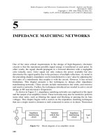
Figure 11.7 A FET-based Clapp oscillator circuit.
456
OSCILLATOR DESIGN
(11.1.27) is satis®ed. An alternative design procedure that provides better stability of
the frequency is as follows. L
3
is selected larger than needed to satisfy (11.1.27), and
then C
B2
is determined to bring it down to the desired value at resonance. This kind
of circuit is called the Clapp oscillator. A FET-based Clapp oscillator circuit is
shown in Figure 11.7. It is very similar to the Colpitts design and operation except
for the selection of C
B2
that is connected in series with the inductor. At the design
frequency, the series inductor-capacitor combination provides the same inductive
reactance as that of the Colpitts circuit. However, if there is a drift in frequency then
the reactance of this combination changes rapidly. This can be explained further with
the help of Figure 11.8.
Figure 11.8 illustrates the resonant circuits of Colpitts and Clapp oscillators. An
obvious difference between the two circuits is the capacitor C
3
that is connected in
series with L
3
. Note that unlike C
3
, the blocking capacitor C
B2
shown in Figure 11.6
does not affect the RF operation.
Reactance X
1
of the series branch in the Colpitts circuit is oL
3
whereas it is
X
2
oL
3
À
1
oC
3
in the case of the Clapp oscillator. If inductor L
3
in the former case
is selected as 1.59 mH and the circuit is resonating at 10 MHz, then the change in its
reactance around resonance is as shown in Figure 11.9. The series branch of the
Clapp circuit has the same inductive reactance at the resonance if L
3
3:18 mH and
C
3
159 pF. However, the rate of change of reactance with frequency is now higher
in comparison with X
1
. This characteristic helps in reducing the drift in oscillation
frequency.
Another Interpretation of the Oscillator Circuit
Ideal inductors and capacitors store electrical energy in the form of magnetic and
electric ®elds, respectively. If such a capacitor with initial charge is connected across
an ideal inductor, it discharges through that. Since there is no loss in this system, the
inductor recharges the capacitor back and the process repeats. However, real
inductors and capacitors are far from being ideal. Energy losses in the inductor
and the capacitor can be represented by a resistance r
1
in this loop. Oscillations die
out because of these losses. As shown in Figure 11.10, if a negative resistance Àr
1
can be introduced in the loop then the effective resistance becomes zero. In other
words, if a circuit can be devised to compensate for the losses then oscillations can
be sustained. This can be done using an active circuit, as illustrated in Figure 11.11.
Figure 11.8 Resonant circuits for Colpitts (a) and Clapp (b) oscillators.
FEEDBACK AND BASIC CONCEPTS
457
Figure 11.10 An ideal oscillator circuit.
Figure 11.9 Reactance of inductive branch versus frequency for Colpitts (X
1
) and Clapp
(X
2
) circuits.
Figure 11.11 A BJT circuit to obtain negative resistance.
458
OSCILLATOR DESIGN
Consider the transistor circuit shown in Figure 11.11. X
1
and X
2
are arbitrary
reactance, and the dc bias circuit is not shown in this circuit for simplicity. For
analysis, a small-signal equivalent circuit can be drawn as illustrated in Figure 11.12.
Using Kirchhoff's voltage law, we can write
V
i
I
i
X
1
X
2
ÀI
b
X
1
À bX
2
11:1:28
and,
0 I
i
X
1
ÀI
b
X
1
r
p
11:1:29
Equation (11.1.29) can be rearranged as follows:
I
b
X
1
X
1
r
p
I
i
11:1:30
Substituting (11.1.30) into (11.1.28), we ®nd that
V
i
I
i
X
1
X
2
À
X
1
À bX
2
X
1
r
p
X
1
11:1:31
Impedance Z
i
across its input terminal can now be determined as follows:
Z
i
V
i
I
i
X
1
X
2
À
X
1
À bX
2
X
1
r
p
X
1
1 bX
1
X
2
X
1
X
2
r
p
X
1
r
p
11:1:32
For X
1
( r
p
, the following approximation can be made
Z
i
%
1 bX
1
X
2
r
p
X
1
X
2
11:1:33
For X
1
and X
2
to be capacitive, it simpli®es to
Z
i
%À
1 b
r
p
Â
1
o
2
C
1
C
2
À j
C
1
C
2
oC
1
C
2
11:1:34
Figure 11.12 A small-signal equivalent of Figure 11.11 with output impedance of the BJT
neglected.
FEEDBACK AND BASIC CONCEPTS
459
Since b, r
p
,andg
m
of a BJT are related as follows:
1 b
r
p
% g
m
(11.1.34) can be further simpli®ed. Hence,
Z
i
%À
g
m
o
2
C
1
C
2
À
j
o
C
1
C
2
C
1
C
2
11:1:35
Therefore, if this circuit is used to replace capacitor C of Figure 11.10 and the
following condition is satis®ed then the oscillations can be sustained
r
1
g
m
o
2
C
1
C
2
11:1:36
The frequency of these oscillations is given as follows:
o
1
LC
1
C
2
C
1
C
2
s
11:1:37
A comparison of this equation with (11.1.27) indicates that it is basically the
Colpitts oscillator. On the other hand, if X
1
and X
2
are inductive then (11.1.33) gives
the following relation
Z
i
%Àg
m
o
2
L
1
L
2
joL
1
L
2
11:1:38
Now, if this circuit replaces inductor L of Figure 11.10 and the following
condition is satis®ed then sustained oscillations are possible
r
1
g
m
o
2
L
1
L
2
11:1:39
The frequency of these oscillations is given as follows:
o
1
CL
1
L
2
p
11:1:40
This is identical to (11.1.26), the Hartley oscillator frequency.
11.2 CRYSTAL OSCILLATORS
Quartz and ceramic crystals are used in the oscillator circuits for additional stability
of frequency. They provide a fairly high Q (of the order of 100,000) that shows a
small drift with temperature (on the order of 0.001 percent per
C). A simpli®ed
electrical equivalent circuit of a crystal is illustrated in Figure 11.13.
460
OSCILLATOR DESIGN
As this equivalent circuit indicates, the crystal exhibits both series and parallel
resonant modes. For example, the terminal impedance of a crystal with typical values
of C
P
29 pF, L
S
58 mH, C
S
0:054 pF, and R
S
15 O exhibits a distinct
minimum and maximum with frequency, as shown in Figure 11.14. Its main
characteristics may be summarized as follows:
Figure 11.13 Equivalent circuit of a crystal.
Figure 11.14 Magnitude (a) and phase angle (b) of the terminal impedance as a function of
frequency.
CRYSTAL OSCILLATORS
461
Magnitude of the terminal impedance decreases up to around 2.844 MHz while
its phase angle remains constant at À90
. Hence, it is effectively a capacitor in
this frequency range.
Magnitude of the impedance dips around 2.844 MHz and its phase angle goes
through a sharp change from À90
to 90
. It has series resonance at this
frequency.
Magnitude of the impedance has a maximum around 2.8465 MHz where its
phase angle changes back to À90
from 90
. It exhibits a parallel resonance
around this frequency.
Phase angle of the impedance remains constant at 90
in the frequency range of
2.844±2.8465 MHz while its magnitude increases. Hence, it is effectively an
inductor.
Beyond 2.8465 MHz, the phase angle stays at À90
while its magnitude goes
down with frequency. Therefore, it is changed back to a capacitor.
Series resonant frequency o
S
and parallel resonant frequency o
P
of the crystal
can be found from its equivalent circuit. These are given as follows:
o
S
1
L
S
C
S
p
11:2:1
and,
o
P
o
S
1
C
S
C
P
s
11:2:2
Hence, the frequency range Do over which the crystal behaves as an inductor can be
determined as follows:
o
P
À o
S
Do o
S
1
C
S
C
P
s
À 1
()
%
C
S
2C
P
o
S
11:2:3
Do is known as the pulling ®gure of the crystal. Typically, o
P
is less than 1
percent higher than o
S
. For an oscillator design, a crystal is selected such that the
frequency of oscillation falls between o
S
and o
P
. Therefore, the crystal operates
basically as an inductor in the oscillator circuit. A BJT oscillator circuit using the
crystal is shown in Figure 11.15. It is known as the Pierce oscillator. A comparison
of its RF equivalent circuit with that shown in Figure 11.4 (b) indicates that the
Pierce circuit is similar to the Colpitts oscillator with inductor L
3
replaced by the
crystal.
As mentioned earlier, the crystal provides very stable frequency of oscillation
over a wide range of temperature. The main drawback of a crystal oscillator circuit is
that its tuning range is relatively small. It is achieved by adding a capacitor in
462
OSCILLATOR DESIGN
parallel with the crystal. This way, the parallel resonant frequency o
P
can be
decreased up to the series resonant frequency o
S
.
11.3 ELECTRONIC TUNING OF OSCILLATORS
In most of the circuits considered so far, capacitance of the tuned circuit can be
varied to change the frequency of oscillation. It can be done electronically by using a
varactor diode and controlling its bias voltage.
There are two basic types of varactorsÐabrupt and hyperabrupt junctions. Abrupt
junction diodes provide very high Q and also operate over a very wide tuning voltage
range (typically, 0 to 60 V). These diodes provide an excellent phase noise
performance because of their high Q.
Hyperabrupt-type diodes exhibit a quadratic characteristic of the capacitance with
applied voltage. Therefore, these varactors provide a much more linear tuning
characteristic than the abrupt type. These diodes are preferred for tuning over a wide
frequency band. An octave tuning range can be covered in less than 20 V. The main
disadvantage of these diodes is that they have a much lower Q, and therefore, the
phase noise is higher than that obtained from the abrupt junction diodes.
The capacitance of a varactor diode is related to its bias voltage as follows:
C
A
V
R
V
B
n
11:3:1
A is a constant; V
R
is the applied reverse bias voltage; and V
B
is the built-in potential
that is 0.7 V for silicon diodes and 1.2 V for GaAs diodes. For the following analysis,
we can write
C
A
V
n
11:3:2
Figure 11.15 Pierce oscillator circuit.
ELECTRONIC TUNING OF OSCILLATORS
463
In this equation, A represents capacitance of the diode when V is one volt. Also, n is
a number between 0.3 and 0.6, but can be as high as 2 for a hyperabrupt junction.
The resonant circuit of a typical voltage-controlled oscillator (VCO) has a parallel
tuned circuit consisting of inductor L, ®xed capacitor C
f
; and the varactor diode with
capacitance C. Therefore, its frequency of oscillation can be written as follows:
o
1
LC
f
C
p
1
LC
f
A
V
n
s
11:3:3
Let o
o
be the angular frequency of an unmodulated carrier and V
o
and C
o
be the
corresponding values of V and C. Then
o
2
o
1
LC
f
C
o
1
LC
f
A
V
n
o
11:3:4
Further, the carrier frequency deviates from o
o
by do for a voltage change of dV .
Therefore,
o
o
do
2
1
LC
f
A
V
o
dV
n
Ao
o
do
À2
LC
f
AV
o
dV
Àn
11:3:5
Dividing (11.3.5) by (11.3.4), we have
o
o
do
o
o
2
C
f
C
o
C
f
AV
o
dV
Àn
C
f
C
o
C
f
AV
Àn
o
1
dV
V
o
Àn
or,
1
do
o
o
2
C
f
C
o
C
f
C
o
1
dV
V
o
Àn
A 1
do
o
o
À2
C
f
C
o
1
dV
V
o
Àn
C
f
C
o
or,
1 À 2
do
o
o
%
C
f
C
o
1 À n
dV
V
o
C
f
C
o
1 À n
dV
V
o
Â
C
o
C
f
C
o
464
OSCILLATOR DESIGN
Hence,
do
dV
no
o
2V
o
C
o
C
f
C
o
!
K
1
11:3:6
K
1
is called the tuning sensitivity of the oscillator. It is expressed in radians per
second per volt.
11.4 PHASE-LOCKED LOOP
Phase-locked loop (PLL) is a feedback system that is used to lock the output
frequency and phase to the frequency and phase of a reference signal at its input. The
reference waveform can be of many different types, including sinusoidal and digital.
The PLL has been used for various applications that include ®ltering, frequency
synthesis, motor speed control, frequency modulation, demodulation, and signal
detection.
The basic PLL consists of a voltage-controlled oscillator (VCO), a phase detector
(PD), and a ®lter. In its most general form, the PLL may also contain a mixer and a
frequency divider as shown in Figure 11.16.
In steady state, the output frequency is expressed as follows:
f
o
f
m
Nf
r
11:4:1
Hence, the output frequency can be controlled by varying N, f
r
,orf
m
.
It is helpful to consider the PLL in terms of phase rather than frequency. This is
done by replacing f
o
, f
m
, f
r
with y
o
, y
m
, and y
r
, respectively. Further, the transfer
characteristics of each building block need to be formulated before the PLL can be
analyzed.
Figure 11.16 Block-diagram of a PLL system.
PHASE-LOCKEDLOOP
465
Phase Detector
With loop in lock, the output of the phase detector is a direct voltage V
e
that is a
function of the phase difference y
d
y
r
À y
f
. If input frequency f
r
is equal to f
f
then
V
e
must be zero. In commonly used analog phase detectors, V
e
is a sinusoidal,
triangular, or sawtooth function of y
d
. It is equal to zero when y
d
is equal to p=2 for
the sinusoidal and triangular types, and p for the sawtooth type. Therefore, it is
convenient to plot V
e
versus a shifted angle y
e
as shown in Figures 11.17±11.19 for a
direct comparison of these three types of detectors. Hence, the transfer characteristic
of a sinusoidal-type phase detector can be expressed as follows:
V
e
A siny
e
À
p
2
y
e
p
2
11:4:2
This can be approximated around y
e
% 0 by the following expression
V
e
% Ay
e
Figure 11.17 Sinusoidal output of the PD.
Figure 11.18 Triangular wave.
466
OSCILLATOR DESIGN
In the case of a triangular output of the phase detector, the transfer characteristic
can be expressed as follows:
V
e
2A
p
y
e
À
p
2
y
e
p
2
11:4:3
From the transfer characteristic of the sawtooth-type phase detector illustrated in
Figure 11.19, we can write
V
e
A
p
y
e
À p y
e
p 11:4:4
Since V
e
is zero in steady state, the gain factor K
d
(volts per radians) in all three
cases is
V
e
y
e
K
d
11:4:5
Voltage-Controlled Oscillator
As described earlier, a varactor diode is generally used in the resonant circuit of an
oscillator. Its bias voltage is controlled to change the frequency of oscillation.
Therefore, the transfer characteristic of an ideal voltage-controlled oscillator (VCO)
has a linear relation, as depicted in Figure 11.20. Hence, the output frequency of a
VCO can be expressed as follows:
f
o
f
S
k
o
V
d
Hz
Figure 11.19 Sawtooth wave.
PHASE-LOCKEDLOOP
467
or,
o
o
o
S
K
o
V
d
radian per sec:
or,
o
o
o
S
do radian per sec:
yt
t
0
o
o
dt o
S
t
t
0
do dt y
S
y
o
t
Therefore,
y
o
t
t
o
do dt A
dy
o
t
dt
do K
o
V
d
11:4:6
In the s-domain,
sy
o
sK
o
V
d
sA
y
o
s
V
d
s
K
o
s
Hence, VCO acts as an integrator.
Loop Filters
A low-pass ®lter is connected right after the phase detector to suppress its output
harmonics. Generally, it is a simple ®rst-order ®lter. Sometimes higher-order ®lters
are also employed to suppress additional ac components. The transfer characteristics
of selected loop-®lters are summarized below.
Figure 11.20 Characteristic of a voltage-controlled oscillator.
468
OSCILLATOR DESIGN
(i) Lead-lag ®lter: A typical lead-lag ®lter uses two resistors and a capacitor, as
illustrated in Figure 11.21. Its transfer function, Fs, can be found as follows:
V
o
V
i
R
2
1
sC
2
R
1
R
2
1
sC
2
1 sR
2
C
2
1 sR
1
C
2
R
2
C
2
Hence,
Fs
1 t
2
s
1 t
1
s
11:4:7
where,
t
2
R
2
C
2
11:4:8
and,
t
1
R
1
R
2
C
2
11:4:9
Typical magnitude and phase characteristics versus frequency (the Bode plot) of a
lead-lag ®lter are illustrated in Figure 11.22. The time constants t
1
and t
2
used to
draw these characteristics were 0.1 s and 0.01 s, respectively. Note that the changes in
these characteristics occur at 1=t
1
and 1=t
2
.
(ii) Integrator and lead ®lter: This kind of ®lter generally requires an OPAMP
along with two resistors and a capacitor. As illustrated in Figure 11.23, the feedback
path of the OPAMP uses a capacitor in series with resistance. Assuming that the
OPAMP is ideal and is being used in inverting con®guration, the transfer character-
istics of this ®lter can be found as follows:
V
o
V
i
À
R
2
1
sC
2
R
1
À
1 sR
2
C
2
sR
1
C
2
Fs
1 st
2
st
1
11:4:10
Figure 11.21 Lead-lag ®lter.
PHASE-LOCKEDLOOP
469
Figure 11.22 Frequency response (Bode plot) of lead-lag ®lter.
Figure 11.23 Integrator and lead ®lter.
470
OSCILLATOR DESIGN
where,
t
1
R
1
C
2
11:4:11
and,
t
2
R
2
C
2
11:4:12
Typical frequency response characteristics (the Bode plot) of an integrator and
lead ®lter are illustrated in Figure 11.24. Time constants t
1
and t
2
used for this
illustration are 0.1 s and 0.01 s, respectively.
Note again that there are signi®cant changes occurring in these characteristics at
frequencies that are equal to 1=t
1
and 1=t
2
. For frequencies less than 10 rad=s phase
angle is almost constant at À90
whereas the magnitude changes at a rate of
20 dB=s. It represents the characteristics of an integrator. Phase angle becomes zero
Figure 11.24 Frequency response (Bode plot) of integrator and lead ®lter.
PHASE-LOCKEDLOOP
471
for frequencies greater than 100 rad=s. The magnitude becomes constant at À20 dB
as well.
(iii) Integrator and lead-lag ®lter: Another active ®lter that is used in the loop is
shown in Figure 11.25. It employs two capacitors in the feedback loop of the
OPAMP. Assuming again that the OPAMP is ideal and is connected in inverting
con®guration, the transfer function of this ®lter can be found as follows:
V
o
V
i
À
1
R
1
R
2
sC
2
R
2
1
sC
2
1
sC
1
0
B
B
@
1
C
C
A
À
1
R
1
R
2
1 sR
2
C
2
1
sC
1
À
R
2
R
1
1 sR
2
C
2
À
1
sR
1
C
1
or,
V
o
V
i
À
sR
2
C
1
1 sR
2
C
2
sR
1
C
1
1 sR
2
C
2
This can be rearranged as follows:
FsÀ
1
st
1
Â
1 st
2
1 st
3
11:4:13
where,
t
1
C
1
R
1
11:4:14
t
2
R
2
C
1
C
2
11:4:15
t
3
R
2
C
2
11:4:16
Frequency response of a typical integrator and lead-lag ®lter is shown in Figure
11.26. Time constants t
1
, t
2
, and t
3
are assumed to be 1, 0.1, and 0.01 s,
respectively. The corresponding frequencies are 1, 10, and 100 rad=s. At frequencies
below 1 rad=s, magnitude of the transfer function reduces at the rate of 20 dB per
decade while its phase angle stays at À90
. Similar characteristics may be observed
higher than 100 rad=s. It is a typical integrator characteristic. Signi®cant change in
the frequency response may be observed at 10 rad=s as well.
An equivalent block diagram of the PLL can be drawn as shown in Figure 11.27.
Output y
o
of the VCO can be controlled by voltage V , reference signal y
r
,or
modulator input y
m
. In order to understand the working of the PLL when it is nearly
locked, the transfer function for each case can be formulated with the help of this
diagram.
472
OSCILLATOR DESIGN
Figure 11.25 Integrator and lead-lag ®lter.
Figure 11.26 Frequency response (Bode plot) of integrator and lead-lag ®lter.
PHASE-LOCKEDLOOP
473