17 linear ODE example k makino
Bạn đang xem bản rút gọn của tài liệu. Xem và tải ngay bản đầy đủ của tài liệu tại đây (121.98 KB, 5 trang )
1. Linear ODE Example - K.Makino
1.1. Preparation. Remainders:
dz
dt
=
f(z,t),z(t)=z(0) +
Z
t
0
f(z,t
0
)dt
0
∂
−1
i
(P
n
+ I
R
)=
Z
x
i
0
P
n−1
dx
i
+ {B(P
n
− P
n−1
)+I
R
}·B(x
i
)
√
3=1.732050808
π/6=0.523598775
(π/6)
5
=0.039354383
1
5!
(π/6)
5
=3.279531944 × 10
−4
1
5!
(π/6)
6
=1.717158911 × 10
−4
1
4!
(π/6)
4
=3.13172232 × 10
−3
1
4!
(π/6)
5
=1.639765972 × 10
−3
The ODEs under consideration are
dx
dt
= −y
dy
dt
= x.
Taylor model identities can be expressed as
i
x
= x
0
+[0, 0],x
0
∈ [−1, 1]
i
y
= y
0
+[0, 0],y
0
∈ [−1, 1].
Let us consider the following initial conditions.
x(t =0)=2+i
x
=2+x
0
+[0, 0]
y(t =0)=0+i
y
= y
0
+[0, 0]
The following calculation is intended t o show the procedures of the algorithms,
and the numbers are not necessarily accurate.
1.2. The First Time Step (t = π/6). The fixed point equations are
x(t)=x(t =0)+
Z
t
0
(−y(t))dt = O
x
(z(t))
y(t)=y(t =0)+
Z
t
0
(x(t))dt = O
y
(z(t)).
The procedures are
• Work on the polynomial part first.
• Find Taylor models satisfying the inclusion requirement.
— Try [0, 0].
— Inflate by 2. (If necessary, repeat the inflation.)
• Refine Taylor models.
1
2
-2
1
1
34
2
y
x
0
x
0
y0
1
-1
-1
0
1
1
1
-1
2
4
3
-1
2
-2
1.2.1. Polynomial Part. Fixed Point Iteration: Step 1
x(t)=2+x
0
+
Z
t
0
[−y
0
] dt =2+x
0
− y
0
t
y(t)=y
0
+
Z
t
0
[2 + x
0
] dt = y
0
+(2+x
0
)t
Fixed Point Iteration: Step 2
x(t)=2+x
0
+
Z
t
0
[−y
0
− (2 + x
0
)t] dt =2+x
0
− y
0
t − (2 + x
0
)
t
2
2
y(t)=y
0
+
Z
t
0
[2 + x
0
− y
0
t] dt = y
0
+(2+x
0
)t − y
0
t
2
2
Fixed Point Iteration: Step
Fixed Point Iteration: Step 5
x(t)=2+x
0
− y
0
t − (2 + x
0
)
t
2
2
+ y
0
t
3
3!
+(2+x
0
)
t
4
4!
− y
0
t
5
5!
y(t)=y
0
+(2+x
0
)t −y
0
t
2
2
− (2 + x
0
)
t
3
3!
+ y
0
t
4
4!
+(2+x
0
)
t
5
5!
Remark: z(t) of a linear system has the linear dependence on the initial condition
z
0
.z(t) of a nonlinear system has the nonlinear dependence on z
0
. For example,
the Volterra equations, dx/dt =2x(1 − y),dy/dt= −y(1 − x), have the nonlinear
dependence on x
0
and y
0
, w hich is not just the second order dependence, but the
high order dependence.
1. LINEAR ODE EXAMPLE - K.MAKINO 3
Thus, for the fifth order computation, we obtain the fifth order polynomial
depending on time t and the initial condition z
0
as a result of the fixed poin t
iteration.
P
x
(x
0
,y
0
,t)=2+x
0
− y
0
t − (2 + x
0
)
t
2
2
+ y
0
t
3
3!
+(2+x
0
)
t
4
4!
P
y
(x
0
,y
0
,t)=y
0
+(2+x
0
)t −y
0
t
2
2
− (2 + x
0
)
t
3
3!
+ y
0
t
4
4!
+2
t
5
5!
(1.1)
1.2.2. Self Inclusion Finding Process. We apply the Picard operation to
x(t)=P
x
(x
0
,y
0
,t)+[0, 0]
y(t)=P
y
(x
0
,y
0
,t)+[0, 0]
using the polynomial solution part (1.1).
x(t)=2+x
0
+
Z
t
0
[−y(t)] dt
= P
x
(x
0
,y
0
,t)+
½
B
µ
−y
0
t
4
4!
+2
t
5
5!
+[0, 0]
¾
· B(t)
= P
x
(x
0
,y
0
,t)+I
(0)
x
y(t)=P
y
(x
0
,y
0
,t)+
½
B
µ
x
0
t
4
4!
+[0, 0]
¾
· B(t)
= P
y
(x
0
,y
0
,t)+I
(0)
y
and we have
I
(0)
x
=[−1.99 × 10
−3
, 1.64 × 10
−3
]
I
(0)
y
=[−1.64 × 10
−3
, 1.64 × 10
−3
].
This provides the guideline to find a self including solution. We inflate it by 2
repeatedly until it satisfies the self i nclusion condition.
I
(1)
x
=2· I
(0)
x
=[−3.97 × 10
−3
, 3.28 × 10
−3
]
I
(1)
y
=2· I
(0)
y
=[−3.28 × 10
−3
, 3.28 × 10
−3
].
Applying the Picard operation, we obtain
I
(1)∗
x
=[−3.71 × 10
−3
, 3.36 × 10
−3
]
I
(1)∗
y
=[−3.72 × 10
−3
, 3.36 × 10
−3
].
I
(2)
x
=2
2
· I
(0)
x
=[−7.94 × 10
−3
, 6.56 × 10
−3
]
I
(2)
y
=2
2
· I
(0)
y
=[−6.56 × 10
−3
, 6.56 × 10
−3
].
I
(2)∗
x
=[−5.42 × 10
−3
, 5.08 × 10
−3
]
I
(2)∗
y
=[−5.80 × 10
−3
, 5.08 × 10
−3
].
Thus, we found a self including solution
P +
I
(2)∗
.
4
(0,0)
34
21
(1,1)
(1,-1)
x
y
0
0
(-1,-1)
(-1,1)
1.2.3. Refinement Process. Now, we apply the Picard operation repeatedly un-
til the desired sharpness of enclosure is achieved.
P +
I
1
= O
³
P +
I
(2)∗
´
=
µ
[−4.64 × 10
−3
, 4.68 × 10
−3
]
[−4.48 × 10
−3
, 4.30 × 10
−3
]
P +
I
2
= O
³
P +
I
1
´
=
µ
[−4.24 × 10
−3
, 3.99 × 10
−3
]
[−4.07 × 10
−3
, 4.09 × 10
−3
]
Con tinuing until the relative tolerance of 1% is met,
P +
I
7
= O
³
P +
I
6
´
=
µ
[−3.84 × 10
−3
, 3.57 × 10
−3
]
[−3.66 × 10
−3
, 3.52 × 10
−3
]
.
1.2.4. Taylor M odel Solution at t = π/6.
x(t = π/6) = P
x
(x
0
,y
0
,t= π/6) + [−3.84 × 10
−3
, 3.57 × 10
−3
]
=1.732 + 0.866x
0
− 0.500y
0
+[−3.84 × 10
−3
, 3.57 × 10
−3
]
y(t = π/6) = P
y
(x
0
,y
0
,t= π/6) + [−3.66 × 10
−3
, 3.52 × 10
−3
]
=1.000 + 0.500x
0
+0.866y
0
+[−3.66 × 10
−3
, 3.52 × 10
−3
](1.2)
Initial position (x
0
,y
0
) at t =0 Mapped position (P
x
,P
y
) at t = π/6
(0,0) (1.732,1.000)
(1,1) (2.098,2.366)
(-1,1) (0.366,1.366)
(-1,-1) (1.366,-0.366)
(1,-1) (3.098,0.634)
1.3. Taylor Model Solution at the Second Time Step (t =2× π/6).
x(t = π/3) = 1.000 + 0.500x
0
− 0.866y
0
+[−1.29 × 10
−2
, 1.26 × 10
−2
]
y(t = π/3) = 1.732 + 0.866x
0
+0.500y
0
+[−1.28 × 10
−2
, 1.24 × 10
−2
]
1. LINEAR ODE EXAMPLE - K.MAKINO 5
1.4. Taylor Model Solution at the Third Time Step (t =3× π/6).
x(t = π/2) = −1.000y
0
+[−3.17 × 10
−2
, 3.16 × 10
−2
]
y(t = π/2) = 2.000 + 1.000x
0
+[−3.20 × 10
−2
, 3.12 × 10
−2
]
1.5. Shrink Wrapping. This is to illustrate the method of shrink w rapping,
andweusethesolutionTaylormodelsatthefirst time step t = π/6.Forthe
simplicity of the argument, we will use sin, cos and so on. From eq. (1.2),
x(t = π/6) =
√
3+cosπ/6 · x
0
− sin π/6 · y
0
+ I
R
x
y(t = π/6) = 1 + sin π/6 · x
0
+cosπ/6 · y
0
+ I
R
y
M(z)=M(z)=
b
A · z + a
where
b
A =
µ
cos π/6 −sin π/6
sin π/6cosπ/6
,a =
µ
√
3
1
,
b
A
−1
=
µ
cos π/6sinπ/6
−sin π/6cosπ/6
so
M
−1
(z)=
b
A
−1
· (z −a)
Thus
M
−1
◦
³
M(z
0
)+
I
R
´
= M
−1
◦
³
M(z
0
)+
I
R
´
=
b
A
−1
·
³
b
A · z
0
+ a +
I
R
−a
´
= z
0
+
b
A
−1
·
I
R
= z
0
+
µ
cos π/6sinπ/6
−sin π/6cosπ/6
¶µ
I
R
x
I
R
y
= z
0
+
µ
0.866 0.500
−0.500 0.866
¶µ
[−3.84 × 10
−3
, 3.57 × 10
−3
]
[−3.66 × 10
−3
, 3.52 × 10
−3
]
= z
0
+
µ
[−5.16 × 10
−3
, 4.86 × 10
−3
]
[−4.96 × 10
−3
, 4.97 × 10
−3
]
µ
[−5.16 × 10
−3
, 4.86 × 10
−3
]
[−4.96 × 10
−3
, 4.97 × 10
−3
]
⊆ 5.16 × 10
−3
·
µ
[−1, 1]
[−1, 1]
≡ d
µ
[−1, 1]
[−1, 1]
.
So, d =5.16 × 10
−3
. The m ap with shrink wrapping is
M
SW
(z
0
)=
b
A(1 + d)z
0
+ a
=(1+5.16 × 10
−3
)
µ
0.866 −0.500
0.500 0.866
¶µ
x
0
y
0
+
µ
1.732
1.000
.