Global optimization for parameter estimation of dynamic systems lin chinese 2005

Global Optimization for Parameter Estimation of
Dynamic Systems
Youdong Lin and Mark A. Stadtherr
Department of Chemical and Biomolecular Engineering
University of Notre Dame
Notre Dame, IN 46556
AIChE Annual Meeting, Cincinnati, OH
October 31, 2005
Outline
• Background
• Interval Analysis
• Taylor Models
• Validated Solutions for Parametric ODEs
• Algorithm Summary
• Computational Studies
• Concluding Remarks and Acknowledgments
2
Background
• Parameter estimation is a key step in development of mathematical models
• Models of interest may be ODEs/DAEs
• Minimization of a weighted squared error
min
θ,z
µ
φ =

m∈M
r

µ=1
(z

µ,m
− ¯z
µ,m
)
2
s.t.
˙
z = f(z, θ, t), z(t
0
) = z
0
θ ∈ Θ
z
µ
= z(t
µ
), t
µ
∈ [t
0
, t
f
]
• Sequential approach – eliminate z
µ
using parametric ODE solver
• Multiple local solutions – a need for global optimization
3
Deterministic Global Optimization with Dynamic Systems
• Much recent interest, e.g.

– Esposito and Floudas (2000)
– Chachuat and Latifi (2003)
– Papamichail and Adjiman (2002, 2004)
– Singer and Barton (2004)
• New approach: branch and reduce algorithm based on interval analysis
– Construct Taylor models of the states using a new validated solver for
parametric ODEs (VSPODE) (Lin and Stadtherr, 2005)
– Compute the Taylor model
T
φ
of the objective function
– Perform constraint propagation procedure using
T
φ
≤
ˆ
φ, to reduce the
parameter domain
4
Interval Analysis
• A real interval
X = [X, X] = {x ∈ R | X ≤ x ≤ X}
• A real interval vector – a box
X = (X
1
, X
2
, · · · , X
n
)

T
• Interval arithmetic – basic operations and elementary functions
• An interval extension of a function f(x) over X
F (X) ⊇ {f(x) | x ∈ X}
• Natural interval extension – leads to overestimation (dependence problem)
5
Taylor Models
• Taylor Model T
f
– an interval extension of a function over X
T
f
= (p
f
, R
f
)
p
f
=
q

i=0
1
i!
[(X − x
0
) · ]
i
f (x

0
)
R
f
=
1
(q+1)!
[(X − x
0
) · ]
q+1
F [x
0
+ (X − x
0
)Ξ]
where,
x
0
∈ X; Ξ = [0, 1]
[g · ]
k
=

j
1
+···+j
m
=k
0≤j

1
,··· ,j
m
≤k
k!
j
1
!···j
m
!
g
j
1
1
· · · g
j
m
m
∂
k
∂x
j
1
1
···∂x
j
m
m
• p
f

is a polynomial function; store and operate on its coefficients only
6
Taylor Models - Remainder Differential Algebra (RDA)
• Basic operations
T
f ±g
= (p
f
, R
f
) ± (p
g
, R
g
) = (p
f
± p
g
, R
f
± R
g
)
T
f ×g
= (p
f
, R
f
) × (p

g
, R
g
)
= p
f
× p
g
+ p
f
× R
g
+ p
g
× R
f
+ R
f
× R
g
= (p
f ×g
, R
f ×g
)
where,
p
f ×g
= p
f

× p
g
− p
e
R
f ×g
= B(p
e
) + B(p
f
) × R
g
+ B(p
g
) × R
f
+ R
f
× R
g
• B(p) indicates an interval bound on the function p.
• Reciprocal operation and intrinsic functions can also be defined.
• It is possible to compute Taylor models of complex functions.
7
Taylor Models - Range Bounding
• Exact range bounding of the interval polynomials – NP hard
• Direct evaluation of the interval polynomials – inefficient
• Focus on bounding the dominant part (1st and 2nd order terms)
• Exact range bounding of a general interval quadratic - computationally
expensive

• A compromise approach – 1st order and diagonal elements of 2nd order
B(p) =
m

i=1

a
i
(X
i
− x
i0
)
2
+ b
i
(X
i
− x
i0
)

+ S
=
m

i=1

a
i


X
i
− x
i0
+
b
i
2a
i

2
−
b
2
i
4a
i

+ S,
where, S is the interval bound of other terms by direct evaluation
8
Taylor Models - Constraint Propagation
• Goal – to reduce part of domain not satisfying c(x) ≤ 0
• For some i = 1, 2 · · · , m
B(T
c
) = B(p
c
) + R

c
= a
i

X
i
− x
i0
+
b
i
2a
i

2
−
b
2
i
4a
i
+ S
i
≤ 0
=⇒ a
i
U
2
i
≤ V

i
, with U
i
= X
i
− x
i0
+
b
i
2a
i
and V
i
=
b
2
i
4a
i
− S
i
=⇒ U
i
=


















∅
if a
i
> 0 and V
i
< 0

−

V
i
a
i
,

V
i
a

i

if a
i
> 0 and V
i
≥ 0
[−∞, ∞]
if a
i
< 0 and V
i
≥ 0

−∞, −

V
i
a
i

∪


V
i
a
i
, ∞


if a
i
< 0 and V
i
< 0
=⇒ X
i
= X
i
∩

U
i
+ x
i0
−
b
i
2a
i

9
Validated Solutions for Parametric ODEs
• Consider the IVP for the parametric ODEs
˙
y = f (y, θ), y(t
0
) = y
0
, θ ∈ Θ

• Validated methods:
– Guarantee there exists a unique solution
y in the interval [t
0
, t
f
], for each
θ ∈ Θ
– Compute the interval Y
t
f
that encloses all solutions of the ODEs at t
f
.
• Tools – AWA, VNODE, COSY VI, VSPODE, etc.
10
Validated Solutions for Parametric ODEs (Cont’d)
• VSPODE (Lin and Stadtherr, 2005) – novel use of Taylor model approach for
dependency problem in solving ODEs with interval valued parameters
• Phase 1 – Validate existence and uniqueness (h
j
and
˜
Y
j
) – like in VNODE
˜
Y
j
=

k−1

i=0
[0, h
j
]
i
F
[i]
(Y
j
, Θ) + [0, h
j
]
k
F
[k]
(
˜
Y
0
j
, Θ) ⊆
˜
Y
0
j
• Phase 2 – Compute tighter enclosure
– Dependence problem – Taylor model
– Wrapping effect – QR factorization

– Solutions:
T
y
j+1
= p
y
j+1
+ A
j+1
V
j+1
11
Validated Solutions for Parametric ODEs (Cont’d)
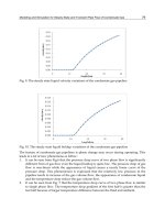
• Example – Lotka-Volterra equations
˙y
1
= θ
1
y
1
(1 − y
2
)
˙y
2
= θ
2
y
2
(y

1
− 1)
t ∈ [0, 10]
y
1
(0) = 1.2
y
2
(0) = 1.1
θ
1
∈ 3 + [−0.01, 0.01]
θ
2
∈ 1 + [−0.01, 0.01]
12
0 1 2 3 4 5 6 7 8 9 10
0.5
0.6
0.7
0.8
0.9
1
1.1
1.2
1.3
1.4
1.5
t
y

1
/y
2
← y
1, VSPODE
← y
2, VSPODE
← y
1, VNODE
← y
2, VNODE
Solution of Lotka−Volterra equations using VSPODE and VNODE
13
Branch and Reduce Algorithm Summary
Beginning with initial parameter interval Θ
(0)
• Establish
ˆ
φ, the upper bound on global minimum using p
2
local minimizations
• Iterate: for subinterval Θ
(k)
1. Compute Taylor models of the states using VSPODE, and then obtain T
φ
2. Perform constraint propagation using T
φ
≤
ˆ
φ to reduce Θ

(k)
3. If Θ
(k)
= ∅, go to next subinterval
4. If
(
ˆ
φ − B(T
φ
))/|
ˆ
φ| ≤ , discard Θ
(k)
and go to next subinterval
5. If
B(T
φ
) <
ˆ
φ, update
ˆ
φ with local minimization, go to step 2
6. If
Θ
(k)
is sufficiently reduced, go to step 1
7. Otherwise, bisect
Θ
(k)
and go to next subinterval

14
Computational Studies - Example 1
• First-order irreversible series reaction (Esposito and Floudas, 2000)
A
θ
1
−→ B
θ
2
−→ C
• The differential equation model
˙z
A
= −θ
1
z
A
˙z
B
= θ
1
z
A
− θ
2
z
B
z
0
= [1, 0]

θ ∈ [0, 10] × [0, 10]
• Solution: θ
∗
= (5.0035, 1.0000) and φ
∗
= 1.1858 × 10
−6
• Results: 4 iterations and < 0.1 CPU seconds
15
Computational Studies - Example 2
• Catalytic Cracking of Gas Oil (Esposito and Floudas, 2000)
A
θ
1
θ
3
Q
θ
2
S
• The differential equation model
˙z
A
= −(θ
1
+ θ
3
)z
2
A

˙z
Q
= θ
1
z
2
A
− θ
2
z
Q
z
0
= [1, 0]
θ ∈ [0, 20] × [0, 20] × [0, 20]
• Solution: θ
∗
= (12.2139, 7.9798, 2.2217) and φ
∗
= 2.6557 × 10
−3
• Results: 359 iterations and 14.3 CPU seconds
16
Computational Performance Comparison (CPU seconds)
Example 1 Example 2
Method Reported Adjusted Reported Adjusted
This work < 0.1 < 0.1 14.3 14.3
(Intel P4 3.2GHz)
Papamichail and Adjiman 801 102.5 35478 4541
(SUN UltraSPARC-II 360MHz)

Chachuat and Latifi 280 - 10400 -
(Machine not reported)
Esposito and Floudas
∗
13.30 1.53 100.21 11.5
(HP 9000 model J2240)
Adjusted = Approximate CPU time adjusted for machine used based on SPEC
benchmarks
∗
Does not provide rigorous guarantee of global optimality.
17
Concluding Remarks and Acknowledgments
• A deterministic global optimization approach based on interval analysis can
be used to estimate the parameters of dynamic systems
• A validated solver for parametric ODEs is used to construct bounds on the
states of dynamic systems
• An efficient constraint propagation procedure is used to reduce the
incompatible parameter domain
• This approach can be combined with the interval-Newton method (Lin and
Stadtherr, 2005)
– True global optimum instead of
-convergence
– May or may not reduce CPU time required
• Acknowledgments
– Indiana 21st Century Research & Technology Fund
– Department of Energy
18