Tài liệu Analog Electronics with Labview P2 ppt
Bạn đang xem bản rút gọn của tài liệu. Xem và tải ngay bản đầy đủ của tài liệu tại đây (156.53 KB, 20 trang )
Unit 3. Characterization of MOS
Transistors for Circuit Simulation
In this unit, the basic (Level 1 SPICE) dc MOSFET characteristic equations are introduced. The
amplifier exercises and projects use the results for design and analysis. Circuit solutions are
compared with measured results from the circuit to make an assessment of the degree to
which the transistor models for the MOSFET represent actual device behavior. The parameters
for this unit are presented in Table 3.1. Note that in the case of KP, we can only measure K
and would be able to extract KP only if gate width W and length L were known.
TABLE 3.1
SPICE Name Math symbol Description
VTO V
tno
, V
tpo
Zero-bias threshold voltage.
KP Transconductance parameter.
Gamma
γ
n
, γ
p
Body-effect parameter.
Phi 2Φ
F
Surface inversion potential.
Lambda λ
n
, λ
p
Channel length modulation.
3.1 Physical Description of the MOSFET
A diagrammatic NMOS is shown in Fig. 3.1. The device consists of a three-layer structure of
metal–oxide–semiconductor (MOS). A two-terminal MOS structure (connections to metal and
semiconductor) is essentially a parallel-plate capacitor. In the same manner as for a normal
capacitor, when a positive gate voltage, V
G
, is applied with respect to the p-type body (for
NMOS) [i.e., with respect to the metal contact on the underside of the p-type semiconductor
body (or substrate)], negative charges are induced under the oxide layer in the semiconductor.
When V
G
(with respect to the semiconductor body) exceeds the threshold voltage, V
tno
, a
channel of free-carrier electrons forms under the oxide; that is, the onset of the channel
occurs when V
G
= V
tno
. The substrate is n type for the PMOS and the channel is made up of
free-carrier holes.
Figure 3.1. MOS transistor consisting of a metal – oxide –
semiconductor layered structure (plus a metal body contact on the
bottom). A positive gate voltage, V
G
> V
tno
, induces a conducting
channel under the oxide, which connects the two n regions, source and
drain. All voltages are with respect to V
B
, that is, the body (substrate)
of the transistor. (a) No channel; (b) uniform channel; (c) channel is
just pinched off at the drain end of the channel; (d) channel length is
reduced due to drain pn-junction depletion region extending out along
the channel.
An n-channel MOSFET device is then completed by fabricating n regions, source and gate, for
contacting the channel on both ends of the channel. For V
G
< V
tno
[Fig. 3.1(a)] there is no
channel under the oxide, and the two n regions are isolated pn junctions. When V
G
> V
tno
and
source voltage, V
S
, and drain voltage, V
D
, are both zero (all with respect to the body) [Fig.
3.1(b)] a uniform-thickness n-type channel exists along the length of the oxide layer and the
source and drain regions are connected by the channel. Thus, the channel is a voltage-
controlled resistor where the two ends of the resistor are at the source and drain and the
control voltage is applied at the gate.
In electronic circuit applications, the terminal voltages are referred to the source; gate and
drain voltages are designated as V
GS
and V
DS
(NMOS). In analog circuits, V
GS
> V
tno
(in order
for a channel to exist), V
DS
is positive, and a drain current flows through the channel and out
by way of the source (and the gate current is zero). On the drain end of the channel, the
voltage across the oxide layer is V
GD
= V
GS
– V
DS
. The channel at the drain end just shuts off
when V
GD
= V
tno
. V
DSsat
= V
GS
– V
tno
[Fig. 3.1(c)] is defined for this condition as the saturation
voltage. The transistor is referred to as in the linear (or triode) region or active region for V
DS
< V
DSsat
and V
DS
> V
DSsat
, respectively.
For V
DS
> V
DSsat
(active mode of operation), the channel length decreases from L to L' as the
reverse-biased depletion region of the drain pn junction increases along the channel (along the
oxide – semiconductor interface) [Fig. 3.1(d)]. The increment V
DS
– V
DSsat
drops across the
depletion region of the drain pn junction. In long-channel devices, the reduction of channel
length is relatively small compared to the channel length. In this case, the length is roughly a
constant and the channel resistance, for a given V
GS
, is independent of V
DS
.
From a circuit point of view, for V
DS
>> V
DSsat
, by Ohm's law,
Equation 3.1
where R
chan
(V
GS
) is the resistance of the channel and is a function of V
GS
. Assuming that L' L,
for a given V
GS
, R
chan
(V
GS
), and thus I
D
, is approximately a constant for V
DS
V
DSsat
. Thus, the
drain, in circuit terms, appears like a current source. In many modern MOSFET devices, this is
only marginally valid. In the following, the definition V
effn
V
DSsat
= V
GS
– V
tno
will be used.
(The subscript is an abbreviation for effective.) The PMOS has a counterpart, V
effp
V
SDsat
=
V
SG
– V
tpo
. V
effp
is a frequently recurring term in device and circuit analytical formulations.
3.2 Output and Transfer Characteristics of the MOSFET
The equations used in the following to characterize the MOSFET transistor are from the SPICE
Level 1 model. SPICE also has more detailed models in Level 2 and Level 3. These can be
specified when running SPICE. However, the number of new model parameters, in general, in
circuit simulation is practically boundless. Level 1 is chosen here as it is the most intuitive, that
is, the most suitable for an introductory discussion of device behavior. Some new models, for
example, which focus on frequency response at very high frequencies, can include pages of
equations. In addition, Level 1 is suitable and adequate for many examples of circuit
simulation.
The basic common-source NMOS circuit configuration is repeated in Fig. 3.2. Here it serves as
a basis for discussing the dc SPICE parameters of the MOSFET transistor. In the example, V
DS
= V
DD
. The output characteristic is a plot of I
D
versus V
DS
for V
GS
= const. A representative
example is shown in Fig. 3.3. As mentioned, the low-voltage region is referred to as the linear
region, triode region, or presaturation region. Outside this region for higher voltages is the
active (saturation) region. This is referred to here as the active region to avoid confusion with
the fact that the nomenclature is just the opposite in the case of the BJT; that is, the low-
voltage region is called the saturation region. As discussed in Unit 3.1, the linear and active
regions are delineated by V
effn
V
DSsat
= V
GS
– V
tno
.
Figure 3.2. Common-source circuit configuration for discussion of the
dc model parameters of the NMOS transistor. The three-terminal
transistor symbol implies that the body and source are connected.
Figure 3.3. Mathcad-generated output characteristic for the NMOS
transistor. The plot illustrates the linear and active regions. The linear
region is also called the triode region or presaturation region. Current
is in microamperes and V
effn
= 0.8 V. Also plotted is the ideal
characteristic with zero slope in the active region.
The output-characteristic equation in the linear region corresponds to V
DS
ranging from the
condition of Fig. 3.1(b) to that of Fig. 3.1
(c). As V
DS
increases from zero, the channel begins to
close off at the drain end (i.e., the channel becomes progressively more wedge shaped). The
result is an increase in the resistance of the channel as a function of V
DS
, and therefore a
sublinear current – voltage relation develops.
When V
GS
> V
tno
, the electron charge in the channel can be related to the gate voltage by Q
chan
= C
ox
(V
GS
– V
tno
) (per unit area of MOSFET looking down at the gate), where C
ox
is the parallel-
plate capacitance (per unit area) formed by the MOS structure. This provides a simple linear
relation between the gate voltage and the charge in the channel.
The conductivity in the channel is σ
chan
= µ
n
Q
chan
/t
chan
, where µ
n
is the mobility of the electrons
in the channel and t
chan
is the thickness of the channel into the semiconductor. Thus, in the
case of a uniform channel (i.e., for V
DS
0), the channel conductance is
Equation 3.2
where
Equation 3.3
and where KP
n
= µ
n
C
ox
is the SPICE transconductance parameter (the n subscript is the
equation symbolic notation for the NMOS; the parameter in the device model is just KP), W is
the physical gate width, and L, again, is the channel length. Parameter KP
n
is related to the
electron mobility in the channel and the oxide thickness. Therefore, it is very specific to a
given MOSFET device.
As V
DS
increases, but is less than V
effn
[transition from Fig. 3.1(b) to 3.1(c)], the wedge-shaped
effect on the channel is reflected functionally in the channel conductance relation as
Equation 3.4
This leads to an output characteristic equation for the linear region, which is
Equation 3.5
The derivation leading to (3.4) and (3.5) is given in Unit 3.4. The linear-region relation, (3.5),
is applicable for V
DS
up to V
DS
= V
effn
, which is the boundary of the linear and active regions.
The active-region equation is then obtained by substituting into (3.5), V
DS
= V
effn
, giving
Equation 3.6
This active-region current corresponds to the zero-slope ideal curve in Fig. 3.3. As discussed in
Unit 3.1, the drain current is not actually constant in the active region (in the same manner as
for a BJT), due to the fact that the physical length of the channel is reduced for increasing V
DS
beyond V
DS
= V
effn
. The reduction in the channel length has the effect of slightly reducing the
resistance of the channel. This is taken into account using the fact that k
n
1/L, from (3.3),
where L is the effective physical length between the source and drain regions. For V
DS
> V
effn
, a
reduced length L' = L(1 – λ
n
V
DS
) is defined which leads to a new effective ,
Equation 3.7
where λ
n
is the SPICE channel-length modulation parameter (Lambda). Substituting for k
n
in
(3.6) produces
Equation 3.8
(Note: A preferred form would be I
D
= k
n
V
effn
2
[1 + λ
n
(V
DS
– V
effn
)] because the channel-length
effect only begins for V
DS
> V
effn
and k
n
could be defined properly for effective length L at V
DS
=
V
effn
. Level 1 SPICE uses (3.8).)
Level 1 SPICE also applies this channel-length reduction factor to the equation in the linear
region, (3.5). To match the linear-region equation to the active-region equation, (3.5
)
becomes, at the edge of the active – linear regions,
Equation 3.9
and, in general
Equation 3.10
[Again, the fact that the channel length is not reduced with the transistor in the linear region
would suggest the use of (3.9) throughout the linear region. Level 1 SPICE uses (3.8
) and
(3.10).]
In general, V
tn
is a function of the source-body voltage, V
SB
. We assume for the moment that
V
SB
= 0. This applies, for example, to the common-source circuit in Fig. 3.2, since the body will
always be at zero volts, and the source in this case is grounded as well. For this case, V
tn
=
V
tno
, as used above. In laboratory projects we measure the output characteristic from which
parameter λ
n
can be obtained. This is based on (3.8). The I – V slope in the active region is
Equation 3.11
From the data measured, a straight-line curve fit determines the slope and the zero V
DS
intercept (I
D
at V
DS
= 0). These are used in (3.11) to obtain λ
n
from λ
n
= slope/intercept. The
intercept is the extension of the active region of Fig. 3.3 (dashed line) to the I
D
axis.
When applying the equations of this development to the PMOS, the voltage between the gate
and source is defined as positive with respect to the source, that is, V
SG
. To be consistent, the
threshold voltage for the PMOS, V
tp
, is also positive. In the SPICE model, however, the
threshold voltage is assigned negative because positive is taken for both types of devices with
respect to the gate (V
GS
is negative for the PMOS), and the threshold voltage for the PMOS is
negative.
The transfer characteristic is obtained by holding V
DS
constant and varying V
GS
. In the MOSFET
parameter-determination experiments of Projects 3 and 4, we plot V
GS
versus for the
transistor biased into the active region. The equation is
Equation 3.12
where is (3.7)
The slope in (3.12) is and the zero intercept is expected to be V
tno
. LabVIEW obtains
the slope and intercept from a straight-line fit to the data. The measured transfer
characteristic thus yields the two parameters
and V
tno
.
In Project 4, parameter λ
n
is obtained from finding at two different V
DS
values. This is based
on
Equation 3.13
where the values are measured and λ
n
is the only unknown.
3.3 Body Effect and Threshold Voltage
In Fig. 3.4 is shown an example of a circuit in which the body and source cannot be at the
same voltage. We now use the four-terminal symbol for the NMOS, which includes the body
contact. In most applications, the body would be tied to the lowest potential in the circuit
(NMOS), in this case, V
SS
(e.g., V
SS
= –5 V). But by the nature of the circuit, the source
voltage is V
S
= V
SS
+ I
D
R
S
, such that the source-body voltage is V
SB
= I
D
R
S
.
Figure 3.4. NMOS transistor circuit with a resistor, R
S
, in the source
branch. With the body attached to V
SS
, V
SB
= I
D
R
S
.
In MOSFET devices, the threshold voltage depends on V
SB
and in SPICE is modeled according
to (NMOS)
Equation 3.14
SPICE parameters contained in the equation are V
tno
(VTO), γ
n
(Gamma), and 2Φ
F
(Phi) (Table
3.1). Typically, γ
n
0.5 V
1/2
and 2Φ
F
0.6 V. Therefore, for example, for V
SB
= 5 V, the body
effect adds 0.8 V to V
tno
.
In the case of the CMOS array ICs of our lab projects (CD4007), the body effect for the PMOS
is significantly less pronounced than for the NMOS (γ
p
< γ
n
), but the parameter for the channel-
length-modulation effect is much smaller for the NMOS than for the PMOS (λ
n
< λ
p
). The
combination suggests that the chip is a p-well configuration; that is, the NMOS devices are
fabricated in "wells" of p-type semiconductor that are fabricated into an n-type substrate. The
PMOS devices reside directly in the n-type substrate material. As far as our measurements are
concerned, the extremes in parameters are an advantage, as we are interested in observing
the effects of the various parameters.
In Project 4, a number for γ
n
is obtained by measuring V
tn
as a function of V
SB
. The results are
plotted as V
tn
versus . LabVIEW calculates the X variable. The data
plotted should give a straight line with slope γ
n
. The effectiveness of SPICE modeling for
representing the behavior of the transistor in a circuit is investigated in Project 4. The transfer
characteristic, V
GS
versus I
D
, is measured for a circuit of the type shown in Fig. 3.4, where the
circuit has V
SB
= I
D
R
S
. In the project, V
SS
is swept over a range of values to produce a range of
I
D
of about a decade. From (3.14), the threshold voltage characteristic that includes the body
effect is
Equation 3.15
The input circuit loop equation (Fig. 3.4) is
Equation 3.16
Including the body effect, V
GS
is now [from (3.12)]
Equation 3.17
where, for this special case, V
DS
= V
GS
(V
D
= 0, V
S
= 0).
A solution is obtainable through combing (3.14), (3.16
), and (3.17) for I
D
and V
GS
. These
equations contain every parameter from this discussion of MOSFET SPICE parameters along
with R
S
. In a project Mathcad file, Project04.mcd, a solution is obtained to provide a
comparison with the measured V
GS
versus I
D
for the circuit. The Mathcad iteration formulation
is, from (3.16),
Equation 3.18
and, from (3.15) and (3.17),
Equation 3.19
I
D
and V
GS
are found for the range of V
SS
corresponding to that used in the measurement,
which is 2.5 < |V
SS
| < 10 V.
3.4 Derivation of the Linear-Region Current – Voltage
Relation
The voltage along the channel is defined as V
c
(x) (Fig. 3.5), with the range 0 at x = 0 (source)
to V
c
(L) = V
D
(drain). The device is in the linear-region mode, that is, V
D
< V
effn
. The charge in
the channel at x is
Equation 3.20
where the charge at the source is Q
chan
= C
ox
(V
GS
– V
tno
), as in the case of (3.2).
Figure 3.5. Diagrammatic NMOS transistor biased into the linear
region.
A generalization of (3.2) for the incremental conductance, dG
chan
(x), at x over a length dx is
Equation 3.21
The voltage drop across the length dx, for a drain current I
D
, is
Equation 3.22
where R
chan
(x) = 1/G
chan
(x). Using (3.21), the incremental voltage across dx is
Equation 3.23
Rearranging the equation and integrating gives
Equation 3.24
which leads to the result (3.5), repeated here
3.5 Summary of Equations
Equations for NMOS. For PMOS, reverse the order of subscripts and define I
D
out of the drain.
Current – voltage relation for the linear region.
Current – voltage relation for the active region.
Threshold-voltage dependence on source-body voltage.
3.6 Exercises and Projects
Project Mathcad Files
Exercise03.mcd - Project03.mcd - Exercise04.mcd, Project04.mcd
Laboratory Project 3
Characterization of the PMOS Transistor for Circuit Simulation
P3.4
Low-Voltage Linear Region of the Output Characteristic
P3.5
PMOS Parameters from the Transfer Characteristic
P3.6
PMOS Lambda from the Transfer Characteristic
P3.7
PMOS Output Characteristic
P3.8
PMOS Lambda
Laboratory Project 4
Characterization of the NMOS Transistor for Circuit Simulation
P4.4
NMOS Parameters from the Transfer Characteristic
P4.5
NMOS Lambda from the Transfer Characteristic
P4.6
NMOS Gamma SubVI
P4.7
NMOS Gamma
P4.8
NMOS Circuit with Body Effect
Unit 4. Signal Conductance Parameters
for Circuit Simulation
The basic low-frequency linear model for a MOS transistor has three conductance parameters:
the transconductance parameter, g
m
, the body-effect parameter, g
mb
, and the output
conductance parameter g
ds
. They are the proportionality constants between incremental
variables of current and voltage. For the linear model to be valid, the increment must be small
compared to the dc (bias) value of the variable. To qualify as small, the increment must be
sufficiently small, in each case, as to avoid unacceptable degrees of nonlinearity in the variable
relationships. The conditions are explored in Unit 5 in connection with linearity of an amplifier
gain function.
In the following, the three conductance parameters are explored, and in each case, an
expression for obtaining the circuit value is developed. The discussion is based on a standard
amplifier stage to provide for an association with electronic circuits.
4.1 Amplifier Circuit and Signal Equivalent Circuits
To serve as an illustration of the utility of the parameters, the discussion of the linear model
and g parameters will be accompanied by a signal-performance evaluation of an NMOS
transistor in the most general amplifier configuration (Fig. 4.1). The circuit includes drain and
source resistors, and input is at the gate terminal. As shown in Fig. 4.1(b), output can be at
the drain (common-source amplifier) or source (source-follower amplifier).
Figure 4.1. (a) Ideal NMOS in a basic common-source amplifier circuit
(output, V
ocs
). Dc supply nodes of Fig. 4.1(a) are set to zero volts to
obtain the signal circuits of Fig. 4.1(b) and (c). An alternative output is
V
oef
[shown in (b)], which is the source-follower amplifier stage.
Voltage variable V
g
is the input for both cases.
Figure 4.1 shows the dc (bias) circuit (a) and signal circuit (b). Replacing all dc nodes with
signal ground and replacing the dc variables with signal variables as in Fig. 4.1 produces the
signal circuit. It will be assumed that the schematic symbol for the transistor in signal circuit
(b) is equivalent to the ideal, intrinsic linear model of the transistor. The total drain current of
the model is I
d
= g
m
V
gs
, as, for example, in the basic circuit of Fig. 2.4. The linear equivalent
model is that of Fig. 4.1(c). The symbolic transistor in Fig. 4.1(b) is more intuitively
representative in terms of the overall circuit perspective than that of Fig. 4.1(c). For this
reason, the Fig. 4.1(b) version is chosen for use in all of the following discussions of MOSFET
circuits. All other details of the transistor model, as discussed in this unit, will be added
externally.
Signal V
g
= V
i
is applied to the gate (input) and, in response, a signal voltage, V
o
, appears at
the drain (or source). We would like to analyze the signal performance in terms of voltage
gain, a
v
= V
o
/V
i
= V
d
/V
g
(or a
v
= V
s
/V
g
), of the circuit based on a linear (small-signal) analysis.
In any case, the voltage gain is a
v
= G
m
R
x
, where G
m
is the circuit transconductance (as
opposed to the transistor transconductance) and x = D (common source) or x = S (source
follower). Thus, the goal will be to obtain a relation for G
m
for a given linear model of the
transistor. Circuit transconductance is determined in the following for models with the various
parameters included.
4.2 Transistor Variable Incremental Relationships
As illustrated previously diagrammatically, for example, in Fig. 3.2, the MOSFET is a four-
terminal device. The four-terminal version of the schematic symbol is repeated here in Fig.
4.2. The terminals again are the source, drain, gate, and body. The drain current and the three
terminal-pair voltages are all interdependent such that i
D
= f(v
DS
, v
GS
, v
SB
). Use of the three-
terminal schematic symbol for the transistor, as in Fig. 4.1, conveys the assumption that the
body and source are connected. For an applied incremental V
gs
, for example, there will be, in
response, incremental drain current I
d
and incremental voltages V
ds
and V
sb
. The linear model
is based on relating the current to the three voltages. This is
Equation 4.1
Figure 4.2. Four-terminal NMOS schematic symbol in a common source
configuration.
The linear-model representation is shown in Fig. 4.3. Figure 4.3(a) shows a current-source
version. The body-effect parameter, g
mb
, is defined as positive. The minus sign is required as
the partial derivative in (4.1) is negative. In Fig. 4.3
(b) the body-effect current source is
reversed to eliminate the minus sign, and the current source associated with g
ds
is replaced
with a resistance. The latter is possible as the voltage-dependent current source is between
the same nodes as the voltage.
Figure 4.3. (a) Linear model that includes all contributions to the
signal drain current, I
d
, as given in (4.1). The body-effect parameter,
g
mb
, is a positive number such that current from the current source is
in the direction opposite the arrow. (b) Current source of body effect is
reversed to eliminate the minus sign, and a resistor replaces the g
ds
current source.
In the following units, using the detailed functions (3.8) and (3.14), which relate the four
variables, expressions, as used in SPICE, will be obtained for the three proportionality
constants: transconductance parameter, g
m
, output conductance parameter, g
ds
, and body-
effect transconductance parameter, g
mb
. The results will be used to obtain numerical results for
the circuit transconductance, G
m
, for various cases.
4.3 Transconductance Parameter
The transconductance parameter, g
m
, was introduced in Unit 2 in the treatment on the
rudimentary electronic amplifier; it is the proportionality constant of the linear relationship
between the output (responding) current and the input (control) voltage [(2.3)]. For the
MOSFET, NMOS, or PMOS, I
d
= g
m
V
gs
, where I
d
is into the drain for both transistor types. An
ideal transistor can be modeled with this alone. A simple model, which includes no other
components, would often be adequate for making estimates of circuit performance.
To obtain an expression for g
m
as a function of the general form i
D
= f(v
GS
, v
DS
, v
SB
) [e.g.,
(3.8)], we use the definition [from (4.1
)]
Equation 4.2
Using (3.8) to express i
D
, the resulting relation for g
m
is
Equation 4.3
where [(3.7)] and V
effn
= V
GS
– V
tno
. Note that the use of V
DS
is consistent
with the partial derivative taken with respect to v
GS
, that is, V
ds
= 0. Also, the use of V
tno
implies that v
SB
= 0. In general, V
SB
could be nonzero, although in the definition of g
m
, V
sb
must be zero. For the case of nonzero V
SB
(bias), one substitutes for V
tno
a constant V
tn
(V
SB
) in
the g
m
expression.
Alternative forms for the g
m
expression can be obtained from (3.8), which is, solving for V
effn
,
Equation 4.4
Using (3.8), (4.3), and (4.4), g
m
takes on altogether three forms:
Equation 4.5
Usually, in initial design, k
n
replaces to eliminate the V
DS
dependence without a serious
penalty in accuracy.