Tài liệu Bài tập về Kinh tế vĩ mô bằng tiếng Anh - Chương 12 doc

Chapter 12: Monopolistic Competition and Oligopoly
191
CHAPTER 12
MONOPOLISTIC COMPETITION AND
OLIGOPOLY

EXERCISES
1. Suppose all firms in a monopolistically competitive industry were merged into one large
firm. Would that new firm produce as many different brands? Would it produce only a
single brand? Explain.
Monopolistic competition is defined by product differentiation. Each firm earns
economic profit by distinguishing its brand from all other brands. This distinction
can arise from underlying differences in the product or from differences in
advertising. If these competitors merge into a single firm, the resulting
monopolist would not produce as many brands, since too much brand competition
is internecine (mutually destructive). However, it is unlikely that only one brand
would be produced after the merger. Producing several brands with different
prices and characteristics is one method of splitting the market into sets of
customers with different price elasticities, which may also stimulate overall
demand.
2. Consider two firms facing the demand curve P = 50 - 5Q, where Q = Q
1
+ Q
2
. The
firms’ cost functions are C
1
(Q
1
) = 20 + 10Q
1

and C
2
(Q
2
) = 10 + 12Q
2
.
a. Suppose both firms have entered the industry. What is the joint profit-maximizing
level of output? How much will each firm produce? How would your answer
change if the firms have not yet entered the industry?
If both firms enter the market, and they collude, they will face a marginal revenue
curve with twice the slope of the demand curve:
MR = 50 - 10Q.
Setting marginal revenue equal to marginal cost (the marginal cost of Firm 1, since
it is lower than that of Firm 2) to determine the profit-maximizing quantity, Q:
50 - 10Q = 10, or Q = 4.
Substituting Q = 4 into the demand function to determine price:
P = 50 – 5*4 = $30.
The question now is how the firms will divide the total output of 4 among
themselves. Since the two firms have different cost functions, it will not be optimal
for them to split the output evenly between them. The profit maximizing solution
is for firm 1 to produce all of the output so that the profit for Firm 1 will be:
π
1
= (30)(4) - (20 + (10)(4)) = $60.
The profit for Firm 2 will be:
π
2
= (30)(0) - (10 + (12)(0)) = -$10.
Chapter 12: Monopolistic Competition and Oligopoly

Total industry profit will be:
π
T
= π
1
+ π
2
= 60 - 10 = $50.
If they split the output evenly between them then total profit would be $46 ($20 for
firm 1 and $26 for firm 2). If firm 2 preferred to earn a profit of $26 as opposed to
$25 then firm 1 could give $1 to firm 2 and it would still have profit of $24, which
is higher than the $20 it would earn if they split output. Note that if firm 2
supplied all the output then it would set marginal revenue equal to its marginal cost
or 12 and earn a profit of 62.2. In this case, firm 1 would earn a profit of –20, so
that total industry profit would be 42.2.
If Firm 1 were the only entrant, its profits would be $60 and Firm 2’s would be 0.

If Firm 2 were the only entrant, then it would equate marginal revenue with its
marginal cost to determine its profit-maximizing quantity:
50 - 10Q
2
= 12, or Q
2
= 3.8.
Substituting Q
2
into the demand equation to determine price:
P = 50 – 5*3.8 = $31.
The profits for Firm 2 will be:
π

2
= (31)(3.8) - (10 + (12)(3.8)) = $62.20.
b. What is each firm’s equilibrium output and profit if they behave noncooperatively?
Use the Cournot model. Draw the firms’ reaction curves and show the equilibrium.
In the Cournot model, Firm 1 takes Firm 2’s output as given and maximizes
profits. The profit function derived in 2.a becomes
π
1
= (50 - 5Q
1
- 5Q
2
)Q
1
- (20 + 10Q
1
), or
π
=
40Q
1
−
5Q
1
2
−
5Q
1
Q
2

−
20.

Setting the derivative of the profit function with respect to Q
1
to zero, we find Firm
1’s reaction function:
∂
π
∂
1
Q
= 40−10
1
Q-5
2
Q=0, or
1
Q=4-
Q
2
2
⎛
⎝
⎞

⎠
.

Similarly, Firm 2’s reaction function is

Q
2
= 3.8−
Q
1
2
⎛
⎝
⎞
⎠
.

To find the Cournot equilibrium, we substitute Firm 2’s reaction function into Firm
1’s reaction function:
Q
1
= 4 −
1
2
⎛
⎝
⎞
⎠
3.8 −
Q
1
2
⎛
⎝
⎞

⎠
, or Q
1
= 2.8.

Substituting this value for Q
1
into the reaction function for Firm 2, we find Q
2
= 2.4.
Substituting the values for Q
1
and Q
2
into the demand function to determine the
equilibrium price:
192
Chapter 12: Monopolistic Competition and Oligopoly
P = 50 – 5(2.8+2.4) = $24.
The profits for Firms 1 and 2 are equal to
π
1
= (24)(2.8) - (20 + (10)(2.8)) = 19.20 and
π
2
= (24)(2.4) - (10 + (12)(2.4)) = 18.80.
c. How much should Firm 1 be willing to pay to purchase Firm 2 if collusion is illegal
but the takeover is not?
In order to determine how much Firm 1 will be willing to pay to purchase Firm 2,
we must compare Firm 1’s profits in the monopoly situation versus those in an

oligopoly. The difference between the two will be what Firm 1 is willing to pay for
Firm 2. From part a, profit of firm 1 when it set marginal revenue equal to its
marginal cost was $60. This is what the firm would earn if it was a monopolist.
From part b, profit was $19.20 for firm 1. Firm 1 would therefore be willing to
pay up to $40.80 for firm 2.

3. A monopolist can produce at a constant average (and marginal) cost of AC = MC = 5.
It faces a market demand curve given by Q = 53 - P.
a. Calculate the profit-maximizing price and quantity for this monopolist. Also
calculate its profits.
The monopolist wants to choose quantity to maximize its profits:
max π = PQ - C(Q),
π = (53 - Q)(Q) - 5Q, or π = 48Q - Q
2
.
To determine the profit-maximizing quantity, set the change in π with respect to
the change in Q equal to zero and solve for Q:
d
dQ
QQ
π
=−+= =2480 24,. or

Substitute the profit-maximizing quantity, Q = 24, into the demand function to find
price:
24 = 53 - P, or P = $29.
Profits are equal to
π = TR - TC = (29)(24) - (5)(24) = $576.
b. Suppose a second firm enters the market. Let Q
1

be the output of the first firm and
Q
2
be the output of the second. Market demand is now given by
Q
1
+ Q
2
= 53 - P.
Assuming that this second firm has the same costs as the first, write the
profits of each firm as functions of Q
1
and Q
2
.
When the second firm enters, price can be written as a function of the output of
two firms: P = 53 - Q
1
- Q
2
. We may write the profit functions for the two firms:
π
1
= PQ
1
− CQ
1
()= 53 −Q
1
− Q

2
()Q
1
− 5Q
1
, or
π
111
2
12 1
53 5=−−−QQQQ Q
193
Chapter 12: Monopolistic Competition and Oligopoly
and
π
2
= PQ
2
− CQ
2
()= 53 − Q
1
− Q
2
()Q
2
− 5Q
2
, or
π

222
2
12 2
53 5=−−−QQQQ Q.
c. Suppose (as in the Cournot model) that each firm chooses its profit-maximizing level
of output on the assumption that its competitor’s output is fixed. Find each firm’s
“reaction curve” (i.e., the rule that gives its desired output in terms of its
competitor’s output).
Under the Cournot assumption, Firm 1 treats the output of Firm 2 as a constant in
its maximization of profits. Therefore, Firm 1 chooses Q
1
to maximize π
1
in b
with Q
2
being treated as a constant. The change in
π
1
with respect to a change in
Q
1
is
∂
π
∂
1
1
12 1
2

53 2 5 0 24
2Q
QQ Q
Q
=− − −= =−,. or

This equation is the reaction function for Firm 1, which generates the profit-
maximizing level of output, given the constant output of Firm 2. Because the
problem is symmetric, the reaction function for Firm 2 is
Q
Q
2
1
24
2
=−.

d. Calculate the Cournot equilibrium (i.e., the values of Q
1
and Q
2
for which both firms
are doing as well as they can given their competitors’ output). What are the
resulting market price and profits of each firm?
To find the level of output for each firm that would result in a stationary
equilibrium, we solve for the values of Q
1
and Q
2
that satisfy both reaction

functions by substituting the reaction function for Firm 2 into the one for Firm 1:
Q
1
= 24 −
1
2
⎛
⎝
⎞

⎠
24 −
Q
1
2
⎛
⎝
⎞

⎠
, or Q
1
= 16.

By symmetry, Q
2
= 16.
To determine the price, substitute Q
1
and Q

2
into the demand equation:
P = 53 - 16 - 16 = $21.
Profits are given by
π
i
= PQ
i
- C(Q
i
) = π
i
= (21)(16) - (5)(16) = $256.
Total profits in the industry are π
1
+ π
2
= $256 +$256 = $512.
*e. Suppose there are N firms in the industry, all with the same constant marginal cost,
MC = 5. Find the Cournot equilibrium. How much will each firm produce, what
will be the market price, and how much profit will each firm earn? Also, show that
as N becomes large the market price approaches the price that would prevail under
perfect competition.
If there are N identical firms, then the price in the market will be

P
=
53
−
Q

1
+
Q
2
+
L
+
Q
N
(
)
.
194
Chapter 12: Monopolistic Competition and Oligopoly
Profits for the i’th firm are given by
π
i
=
PQ
i
−
CQ
i
(
)
,

π
i
= 53Q

i
− Q
1
Q
i
−
Q
2
Q
i
−
L
−
Q
i
2
−
L
−
Q
N
Q
i
−
5Q
i
.
Differentiating to obtain the necessary first-order condition for profit maximization,
d
dQ

QQQ
i
iN
π
= − −− −− −=53 2 5 0
1
LL
.
Solving for Q
i
,

Q
i
= 24−
1
2
Q
1
+L + Q
i−1
+ Q
i+1
+L + Q
N
()
.
If all firms face the same costs, they will all produce the same level of output, i.e.,
Q
i

= Q*. Therefore,
Q* = 24−
1
2
N − 1()Q*, or 2Q* = 48− N −1()Q*, or

N +1()Q* = 48, or Q* =
48
N + 1
()
.

We may substitute for Q = NQ*, total output, in the demand function:
P = 53− N
48
N +1
⎛
⎝
⎞

⎠
.


Total profits are
π
T
= PQ - C(Q) = P(NQ*) - 5(NQ*)
or
π

T

= 53 − N
48
N
+ 1
⎛
⎝
⎞

⎠
⎡
⎣
⎢
⎤
⎦
⎥
N
()
48
N
+ 1
⎛
⎝
⎞

⎠
− 5N
48
N

+1
⎛
⎝
⎞

⎠

or
π
T

= 48 − N
()
48
N
+ 1
⎛
⎝
⎞

⎠
⎡

⎣
⎢
⎤
⎦
⎥
N
()

48
N
+ 1
⎛
⎝
⎞

⎠


or
π
T

= 48
()
N + 1− N
N + 1
⎛
⎝
⎞
⎠
48
()
N
N +1
⎛
⎝
⎞
⎠

= 2, 304
()
N
N + 1
()
2
⎛
⎝
⎞

⎠
.

Notice that with N firms
Q = 48
N
N
+ 1
⎛
⎝
⎞

⎠

and that, as N increases (N → ∞)
Q = 48.
Similarly, with
P = 53 − 48
N
N

+ 1
⎛
⎝
⎞

⎠
,

as N → ∞,
195
Chapter 12: Monopolistic Competition and Oligopoly
P = 53 - 48 = 5.
With P = 5, Q = 53 - 5 = 48.
Finally,
π
T
= 2,304
N
N +1
()
2
⎛
⎝
⎜
⎞

⎠
⎟
,

so as N → ∞,
π
T
= $0.
In perfect competition, we know that profits are zero and price equals marginal
cost. Here, π
T
= $0 and P = MC = 5. Thus, when N approaches infinity, this
market approaches a perfectly competitive one.
4. This exercise is a continuation of Exercise 3. We return to two firms with the same
constant average and marginal cost, AC = MC = 5, facing the market demand curve
Q
1
+ Q
2
= 53 - P. Now we will use the Stackelberg model to analyze what will happen if one
of the firms makes its output decision before the other.
a. Suppose Firm 1 is the Stackelberg leader (i.e., makes its output decisions before Firm
2). Find the reaction curves that tell each firm how much to produce in terms of the
output of its competitor.

Firm 1, the Stackelberg leader, will choose its output, Q
1
, to maximize its profits,
subject to the reaction function of Firm 2:
max π
1
= PQ
1
- C(Q

1
),
subject to
Q
2
= 24 −
Q
1
2
⎛
⎝
⎞

⎠
.


Substitute for Q
2
in the demand function and, after solving for P, substitute for P in
the profit function:
max
π
1
= 53− Q
1
− 24 −
Q
1
2

⎛
⎝
⎞

⎠
⎛
⎝
⎞

⎠
Q
1
()− 5Q
1
.

To determine the profit-maximizing quantity, we find the change in the profit
function with respect to a change in Q
1
:
d
dQ
QQ
π
1
1
11
53 2 24 5=− −+−.

Set this expression equal to 0 to determine the profit-maximizing quantity:

53 - 2Q
1
- 24 + Q
1
- 5 = 0, or Q
1
= 24.
Substituting Q
1
= 24 into Firm 2’s reaction function gives Q
2
:
Q
2
24
24
2
12=− =.

Substitute Q
1
and Q
2
into the demand equation to find the price:
196
Chapter 12: Monopolistic Competition and Oligopoly
P = 53 - 24 - 12 = $17.
Profits for each firm are equal to total revenue minus total costs, or
π
1

= (17)(24) - (5)(24) = $288 and
π
2
= (17)(12) - (5)(12) = $144.
Total industry profit, π
T
= π
1
+ π
2
= $288 + $144 = $432.
Compared to the Cournot equilibrium, total output has increased from 32 to 36,
price has fallen from $21 to $17, and total profits have fallen from $512 to $432.
Profits for Firm 1 have risen from $256 to $288, while the profits of Firm 2 have
declined sharply from $256 to $144.
b. How much will each firm produce, and what will its profit be?
If each firm believes that it is the Stackelberg leader, while the other firm is the
Cournot follower, they both will initially produce 24 units, so total output will be
48 units. The market price will be driven to $5, equal to marginal cost. It is
impossible to specify exactly where the new equilibrium point will be, because no
point is stable when both firms are trying to be the Stackelberg leader.
5. Two firms compete in selling identical widgets. They choose their output levels Q
1

and Q
2
simultaneously and face the demand curve
P = 30 - Q,
where Q = Q
1

+ Q
2
. Until recently, both firms had zero marginal costs. Recent
environmental regulations have increased Firm 2’s marginal cost to $15. Firm 1’s
marginal cost remains constant at zero. True or false: As a result, the market price will
rise to the monopoly level.
True.
If only one firm were in this market, it would charge a price of $15 a unit. Marginal
revenue for this monopolist would be
MR = 30 - 2Q,
Profit maximization implies MR = MC, or
30 - 2Q = 0, Q = 15, (using the demand curve) P = 15.
The current situation is a Cournot game where Firm 1's marginal costs are zero and Firm
2's marginal costs are 15. We need to find the best response functions:
Firm 1’s revenue is
PQ
1
= (30
−
Q
1
−
Q
2
)Q
1
=
30Q
1
−

Q
1
2
−
Q
1
Q
2
,

and its marginal revenue is given by:
M
R
1
=
30
−
2Q
1
−
Q
2
.

Profit maximization implies MR
1
= MC
1
or
30 − 2Q

1
− Q
2
= 0 ⇒ Q
1
=15−
Q
2
2
,

which is Firm 1’s best response function.
197
Chapter 12: Monopolistic Competition and Oligopoly
Firm 2’s revenue function is symmetric to that of Firm 1 and hence
M
R
2
=
30
−
Q
1
−
2Q
2
.

Profit maximization implies MR
2

= MC
2
, or
30 − 2Q
2
− Q
1
= 15⇒ Q
2
= 7.5 −
Q
1
2
,

which is Firm 2’s best response function.
Cournot equilibrium occurs at the intersection of best response functions. Substituting
for Q
1
in the response function for Firm 2 yields:
Q
2
= 7.5− 0.5(15 −
Q
2
2
).

Thus Q
2

=0 and Q
1
=15. P = 30 - Q
1
+ Q
2
= 15, which is the monopoly price.
6. Suppose that two identical firms produce widgets and that they are the only firms in the
market. Their costs are given by C
1
= 60Q
1
and C
2
= 60Q
2
, where Q
1
is the output of Firm
1 and Q
2
the output of Firm 2. Price is determined by the following demand curve:
P = 300 - Q
where Q = Q
1
+ Q
2
.
a. Find the Cournot-Nash equilibrium. Calculate the profit of each firm at this
equilibrium.

To determine the Cournot-Nash equilibrium, we first calculate the reaction
function for each firm, then solve for price, quantity, and profit. Profit for Firm 1,
TR
1
- TC
1
, is equal to
π
1
= 300Q
1
− Q
1
2
−
Q
1
Q
2
−
60Q
1
=
240Q
1
−
Q
1
2
−

Q
1
Q
2
.

Therefore,
∂
1
π
∂
1
Q
= 240 − 2
1
Q −
2
Q.

Setting this equal to zero and solving for Q
1
in terms of Q
2
:
Q
1
= 120 - 0.5Q
2
.
This is Firm 1’s reaction function. Because Firm 2 has the same cost structure,

Firm 2’s reaction function is
Q
2
= 120 - 0.5Q
1
.
Substituting for Q
2
in the reaction function for Firm 1, and solving for Q
1
, we find
Q
1
= 120 - (0.5)(120 - 0.5Q
1
), or Q
1
= 80.
By symmetry, Q
2
= 80. Substituting Q
1
and Q
2
into the demand equation to
determine the price at profit maximization:
P = 300 - 80 - 80 = $140.
Substituting the values for price and quantity into the profit function,
π
1

= (140)(80) - (60)(80) = $6,400 and
198
Chapter 12: Monopolistic Competition and Oligopoly
π
2
= (140)(80) - (60)(80) = $6,400.
Therefore, profit is $6,400 for both firms in Cournot-Nash equilibrium.
b. Suppose the two firms form a cartel to maximize joint profits. How many widgets
will be produced? Calculate each firm’s profit.

Given the demand curve is P=300-Q, the marginal revenue curve is MR=300-2Q.
Profit will be maximized by finding the level of output such that marginal revenue
is equal to marginal cost:
300-2Q=60
Q=120.
When output is equal to 120, price will be equal to 180, based on the demand
curve. Since both firms have the same marginal cost, they will split the total
output evenly between themselves so they each produce 60 units. Profit for each
firm is:
π = 180(60)-60(60)=$7,200.
Note that the other way to solve this problem, and arrive at the same solution is to
use the profit function for either firm from part a above and let
Q
=
Q
1
= Q
2
.
c. Suppose Firm 1 were the only firm in the industry. How would the market output

and Firm 1’s profit differ from that found in part (b) above?
If Firm 1 were the only firm, it would produce where marginal revenue is equal to
marginal cost, as found in part b. In this case firm 1 would produce the entire 120
units of output and earn a profit of $14,400.
d. Returning to the duopoly of part (b), suppose Firm 1 abides by the agreement, but
Firm 2 cheats by increasing production. How many widgets will Firm 2 produce?
What will be each firm’s profits?
Assuming their agreement is to split the market equally, Firm 1 produces 60
widgets. Firm 2 cheats by producing its profit-maximizing level, given Q
1
= 60.
Substituting
Q
1
= 60 into Firm 2’s reaction function:
Q
2
= 120−
60
2
= 90.

Total industry output, Q
T
, is equal to Q
1
plus Q
2
:
Q

T
= 60 + 90 = 150.
Substituting Q
T
into the demand equation to determine price:
P = 300 - 150 = $150.

199
Chapter 12: Monopolistic Competition and Oligopoly
200
Substituting Q
1
, Q
2
, and P into the profit function:
π
1
= (150)(60) - (60)(60) = $5,400 and
π
2
= (150)(90) - (60)(90) = $8,100.
Firm 2 has increased its profits at the expense of Firm 1 by cheating on the
agreement.
7. Suppose that two competing firms, A and B, produce a homogeneous good. Both firms
have a marginal cost of MC=$50. Describe what would happen to output and price in each
of the following situations if the firms are at (i) Cournot equilibrium, (ii) collusive
equilibrium, and (iii) Bertrand equilibrium.
a. Firm A must increase wages and its MC increases to $80.
(i) In a Cournot equilibrium you must think about the effect on the reaction
functions, as illustrated in figure 12.4 of the text. When firm A experiences an

increase in marginal cost, their reaction function will shift inwards. The quantity
produced by firm A will decrease and the quantity produced by firm B will increase.
Total quantity produced will tend to decrease and price will increase.
(ii) In a collusive equilibrium, the two firms will collectively act like a
monopolist. When the marginal cost of firm A increases, firm A will reduce their
production. This will increase price and cause firm B to increase production.
Price will be higher and total quantity produced will be lower.
(iii) Given that the good is homogeneous, both will produce where price equals
marginal cost. Firm A will increase price to $80 and firm B will keep its price at
$50. Assuming firm B can produce enough output, they will supply the entire
market.

b. The marginal cost of both firms increases.
(i) Again refer to figure 12.4. The increase in the marginal cost of both firms
will shift both reaction functions inwards. Both firms will decrease quantity
produced and price will increase.
(ii) When marginal cost increases, both firms will produce less and price will
increase, as in the monopoly case.
(iii) As in the above cases, price will increase and quantity produced will
decrease.

c. The demand curve shifts to the right.
(i) This is the opposite of the above case in part b. In this case, both reaction
functions will shift outwards and both will produce a higher quantity. Price will
tend to increase.
(ii) Both firms will increase the quantity produced as demand and marginal
revenue increase. Price will also tend to increase.
(iii) Both firms will supply more output. Given that marginal cost is constant,
the price will not change.

8. Suppose the airline industry consisted of only two firms: American and Texas Air Corp.
Let the two firms have identical cost functions, C(q) = 40q. Assume the demand curve for
Chapter 12: Monopolistic Competition and Oligopoly
the industry is given by P = 100 - Q and that each firm expects the other to behave as a
Cournot competitor.
a. Calculate the Cournot-Nash equilibrium for each firm, assuming that each chooses
the output level that maximizes its profits when taking its rival’s output as given.
What are the profits of each firm?

To determine the Cournot-Nash equilibrium, we first calculate the reaction
function for each firm, then solve for price, quantity, and profit. Profit for Texas
Air, π
1
, is equal to total revenue minus total cost:

π
1
= (100 - Q
1
- Q
2
)Q
1
- 40Q
1
, or
ππ
111
2
12 1 1 1 1

2
12
100 40 60=−−− =−−QQ QQ Q QQ QQ,. or
The change in π
1
with respect to Q
1
is
∂
∂
=− −
1
1
12
60 2
π
Q
QQ
.

Setting the derivative to zero and solving for Q
1
in terms of Q
2
will give Texas Air’s
reaction function:
Q
1
= 30 - 0.5Q
2

.
Because American has the same cost structure, American’s reaction function is
Q
2
= 30 - 0.5Q
1
.
Substituting for Q
2
in the reaction function for Texas Air,
Q
1
= 30 - 0.5(30 - 0.5Q
1
) = 20.
By symmetry, Q
2
= 20. Industry output, Q
T
, is Q
1
plus Q
2
, or
Q
T
= 20 + 20 = 40.
Substituting industry output into the demand equation, we find P = 60.
Substituting Q
1

, Q
2
, and P into the profit function, we find
π
1
= π
2
= 60(20) -20
2
- (20)(20) = $400
for both firms in Cournot-Nash equilibrium.
b. What would be the equilibrium quantity if Texas Air had constant marginal and
average costs of $25, and American had constant marginal and average costs of $40?

By solving for the reaction functions under this new cost structure, we find that
profit for Texas Air is equal to
π
111
2
12 1 1 1
2
12
100 25 75=−−−=−−QQ QQ Q QQ QQ.
The change in profit with respect to Q
1
is
∂
∂
=− −
π

1
1
12
75 2
Q
QQ
.

201
Set the derivative to zero, and solving for Q
1
in terms of Q
2
,
Chapter 12: Monopolistic Competition and Oligopoly
202
Q
1
= 37.5 - 0.5Q
2
.
This is Texas Air’s reaction function. Since American has the same cost structure
as in 8.a., American’s reaction function is the same as before:
Q
2
= 30 - 0.5Q
1
.
To determine Q
1

, substitute for Q
2
in the reaction function for Texas Air and solve
for Q
1
:
Q
1
= 37.5 - (0.5)(30 - 0.5Q
1
) = 30.
Texas Air finds it profitable to increase output in response to a decline in its cost
structure.
To determine Q
2
, substitute for Q
1
in the reaction function for American:
Q
2
= 30 - (0.5)(37.5 - 0.5Q
2
) = 15.
American has cut back slightly in its output in response to the increase in output by
Texas Air.
Total quantity, Q
T
, is Q
1
+ Q

2
, or
Q
T
= 30 + 15 = 45.
Compared to 8a, the equilibrium quantity has risen slightly.
c. Assuming that both firms have the original cost function, C(q) = 40q, how much
should Texas Air be willing to invest to lower its marginal cost from $40 to $25,
assuming that American will not follow suit? How much should American be
willing to spend to reduce its marginal cost to $25, assuming that Texas Air will have
marginal costs of $25 regardless of American’s actions?
Recall that profits for both firms were $400 under the original cost structure.
With constant average and marginal costs of 25, Texas Air’s profits will be
(55)(30) - (25)(30) = $900.
The difference in profit is $500. Therefore, Texas Air should be willing to invest
up to $500 to lower costs from 40 to 25 per unit (assuming American does not
follow suit).
To determine how much American would be willing to spend to reduce its average
costs, we must calculate the difference in profits, assuming Texas Air’s average
cost is 25. First, without investment, American’s profits would be:
(55)(15) - (40)(15) = $225.
Second, with investment by both firms, the reaction functions would be:
Q
1
= 37.5 - 0.5Q
2
and
Q
2
= 37.5 - 0.5Q

1
.
To determine Q
1
, substitute for Q
2
in the first reaction function and solve for Q
1
:
Q
1
= 37.5 - (0.5)(37.5 - 0.5Q
1
) = 25.
Substituting for Q
1
in the second reaction function to find Q
2
:
Chapter 12: Monopolistic Competition and Oligopoly
203
Q
2
= 37.5 - 0.5(37.5 - 0.5Q
2
) = 25.
Substituting industry output into the demand equation to determine price:
P = 100 - 50 = $50.
Therefore, American’s profits if Q
1

= Q
2
= 25 (when both firms have MC = AC =
25) are
π
2
= (100 - 25 - 25)(25) - (25)(25) = $625.
The difference in profit with and without the cost-saving investment for American
is $400. American would be willing to invest up to $400 to reduce its marginal
cost to 25 if Texas Air also has marginal costs of 25.
Chapter 12: Monopolistic Competition and Oligopoly
*9. Demand for light bulbs can be characterized by Q = 100 - P, where Q is in millions of
lights sold, and P is the price per box. There are two producers of lights: Everglow and
Dimlit. They have identical cost functions:

C
i
= 10Q
i
+ 1/ 2Q
i
2
i
=
E, D()
i
i
Q = Q
E
+ Q

D
.
a. Unable to recognize the potential for collusion, the two firms act as short-run perfect
competitors. What are the equilibrium values of Q
E
, Q
D
, and P? What are each
firm’s profits?
Given that the total cost function is , the marginal cost curve for
each firm is
. In the short run, perfectly competitive firms
determine the optimal level of output by taking price as given and setting price
equal to marginal cost. There are two ways to solve this problem. One way is to
set price equal to marginal cost for each firm so that:
CQ Q
ii
=+10 1 2
2
/
MC Q
i
=+10
P
=
100
−
Q
1
−

Q
2
=
10
+
Q
1
P = 100− Q
1
− Q
2
=10 + Q
2
.

Given we now have two equations and two unknowns, we can solve for Q
1
and Q
2
.
Solve the second equation for Q
2
to get
Q
2
=
90
−
Q
1

2
,

and substitute into the other equation to get
100 − Q
1
−
90
−
Q
1
2
=10 + Q
1
.

This yields a solution where Q
1
=30, Q
2
=30, and P=40. You can verify that
P=MC for each firm. Profit is total revenue minus total cost or
Π=40 * 30 − (10 *30
+
0.5*30*30)
=
$450 million.

The other way to solve the problem and arrive at the same solution is to find the
market supply curve by summing the marginal cost curves, so that Q

M
=2P-20 is the
market supply. Setting supply equal to demand results in a quantity of 60 in the
market, or 30 per firm since they are identical.
b. Top management in both firms is replaced. Each new manager independently
recognizes the oligopolistic nature of the light bulb industry and plays Cournot.
What are the equilibrium values of Q
E
, Q
D
, and P? What are each firm’s profits?
To determine the Cournot-Nash equilibrium, we first calculate the reaction
function for each firm, then solve for price, quantity, and profit. Profits for
Everglow are equal to TR
E
- TC
E
, or
π
E
= 100 − Q
E
− Q
D
()Q
E
− 10Q
E
+ 0.5Q
E

2
(
)
= 90Q
E
− 1.5Q
E
2
− Q
E
Q
D
.

The change in profit with respect to Q
E
is
∂
∂
−−
π
E
E
ED
Q
=
QQ
.90 3

204

Chapter 12: Monopolistic Competition and Oligopoly
To determine Everglow’s reaction function, set the change in profits with respect
to Q
E
equal to 0 and solve for Q
E
:
90 - 3Q
E
- Q
D
= 0, or
Q
E
=
90
−
Q
D
3
.

Because Dimlit has the same cost structure, Dimlit’s reaction function is
Q
D
=
90
−
Q
E

3
.

Substituting for Q
D
in the reaction function for Everglow, and solving for Q
E
:
Q
E
=
90 −
90
−
Q
E
3
3
3Q
E
= 90 − 30+
Q
E
3
Q
E
= 22.5.

By symmetry, Q
D

= 22.5, and total industry output is 45.
Substituting industry output into the demand equation gives P:
45 = 100 - P, or P = $55.
Substituting total industry output and P into the profit function:
Π
i
= 22.5*55− (10 * 22.5
+
0.5*22.5*22.5)
=
$759.375 million.

c. Suppose the Everglow manager guesses correctly that Dimlit has a Cournot
conjectural variation, so Everglow plays Stackelberg. What are the equilibrium
values of Q
E
, Q
D
, and P? What are each firm’s profits?
Recall Everglow’s profit function:
π
E
= 100− Q
E
− Q
D
() Q
E
− 10Q
E

+0.5Q
E
2
(
)
.

If Everglow sets its quantity first, knowing Dimlit’s reaction function
i.e., Q
D
= 30 −
Q
E
3
⎛
⎝
⎞

⎠

, we may determine Everglow’s reaction function by substituting for
Q
D
in its profit function. We find
π
EE
E
Q
Q
=−60

7
6
2
.
To determine the profit-maximizing quantity, differentiate profit with respect to
Q
E
, set the derivative to zero and solve for Q
E
:
∂
∂
=− = =
π
E
E
E
E
Q
Q
,
Q
60
7
3
02or
57

Substituting this into Dimlit’s reaction function, we find
Q

D
=− =30
25 7
3
21 4
.


Total industry output is 47.1 and P = $52.90. Profit for Everglow is $772.29
million. Profit for Dimlit is $689.08 million.
205
Chapter 12: Monopolistic Competition and Oligopoly
d. If the managers of the two companies collude, what are the equilibrium values of Q
E
,
Q
D
, and P? What are each firm’s profits?
If the firms split the market equally, total cost in the industry is
10
2
2
Q
Q
T
T
+
;
therefore, . Total revenue is
100

MC Q
T
=+10
Q
T
−
Q
T
2
; therefore,
M
R = 100 − 2Q
T
.
To determine the profit-maximizing quantity, set MR = MC and
solve for Q
T
:
100
−
2Q
T
=
10
+
Q
T
, or Q
T
=

30.

This means Q
E
= Q
D
= 15.
Substituting Q
T
into the demand equation to determine price:
P = 100 - 30 = $70.
The profit for each firm is equal to total revenue minus total cost:
π
i
= 70()15()− 10()15()+
15
2
2
⎛
⎝
⎜
⎞

⎠
⎟
= $787.50 million.

10. Two firms produce luxury sheepskin auto seat covers, Western Where (WW) and
B.B.B. Sheep (BBBS). Each firm has a cost function given by:
C (q) = 30q + 1.5q

2
The market demand for these seat covers is represented by the inverse demand equation:
P = 300 - 3Q,
where Q = q
1
+ q
2
, total output.
a. If each firm acts to maximize its profits, taking its rival’s output as given (i.e., the
firms behave as Cournot oligopolists), what will be the equilibrium quantities
selected by each firm? What is total output, and what is the market price? What
are the profits for each firm?
We are given each firm’s cost function C(q) = 30q + 1.5q
2
and the market
demand function P = 300 - 3Q where total output Q is the sum of each firm’s
output q
1
and q
2.
We find the best response functions for both firms by setting
marginal revenue equal to marginal cost (alternatively you can set up the profit
function for each firm and differentiate with respect to the quantity produced for
that firm):
R
1
= P q
1
= (300 - 3(q
1

+ q
2
)) q
1
= 300q
1
- 3q
1
2
- 3q
1
q
2
.

MR
1
= 300 - 6q
1
- 3q
2
MC
1
= 30 + 3q
1
300 - 6q
1
- 3q
2
= 30 + 3q

1

q
1
= 30 - (1/3)q
2
.

By symmetry, BBBS’s best response function will be:
206
Chapter 12: Monopolistic Competition and Oligopoly
207
q
2
= 30 - (1/3)q
1
.

Cournot equilibrium occurs at the intersection of these two best response
functions, given by:
q
1
= q
2
= 22.5.
Thus,
Q = q
1
+ q
2

= 45
P = 300 - 3(45) = $165.
Profit for both firms will be equal and given by:
R - C = (165) (22.5) - (30(22.5) + 1.5(22.5
2
)) = $2278.13.
b. It occurs to the managers of WW and BBBS that they could do a lot better by
colluding. If the two firms collude, what would be the profit-maximizing choice of
output? The industry price? The output and the profit for each firm in this case?
If firms can collude, then in this case they should each produce half the quantity
that maximizes total industry profits (i.e. half the monopoly profits). If on the
other hand the two firms had different cost functions, then it would not be optimal
for them to split the monopoly output evenly.
Joint profits will be (300-3Q)Q - 2(30(Q/2) + 1.5(Q/2)
2
) = 270Q - 3.75Q
2
and will
be maximized at Q = 36. You can find this quantity by differentiating the above
profit function with respect to Q, setting the resulting first order condition equal
to zero, and then solving for Q.
Thus, we will have q
1
= q
2
= 36 / 2 = 18 and P = 300 - 3(36) = $192.
Profit for each firm will be 18(192) - (30(18) + 1.5(18
2
)) = $2,430.
c. The managers of these firms realize that explicit agreements to collude are illegal.

Each firm must decide on its own whether to produce the Cournot quantity or the
cartel quantity. To aid in making the decision, the manager of WW constructs a
payoff matrix like the real one below. Fill in each box with the (profit of WW,
profit of BBBS). Given this payoff matrix, what output strategy is each firm likely
to pursue?
If WW produces the Cournot level of output (22.5) and BBBS produces the
collusive level (18), then:
Q = q
1
+ q
2
= 22.5 + 18 = 40.5
P = 300 -3(40.5) = $178.5.
Profit for WW = 22.5(178.5) - (30(22.5) + 1.5(22.5
2
)) = $2581.88.
Profit for BBBS = 18(178.5) - (30(18) + 1.5(18
2
)) = $2187.
Both firms producing at the Cournot output levels will be the only Nash
Equilibrium in this industry, given the following payoff matrix. Given the firms
end up in any other cell in the matrix, one of them will always have an incentive
to change their level of production in order to increase profit. For example, if
WW is Cournot and BBBS is cartel, then BBBS has an incentive to switch to
Chapter 12: Monopolistic Competition and Oligopoly
cartel to increase profit. (Note: not only is this a Nash Equilibrium, but it is an
equilibrium in dominant strategies.)

Profit Payoff Matrix BBBS

(WW profit, BBBS
profit)
Produce
Cournot
q
Produce
Cartel q


WW
Produce
Cournot
q
2278,2278 2582, 2187

Produce
Cartel q
2187, 2582 2430,2430
d. Suppose WW can set its output level before BBBS does. How much will WW
choose to produce in this case? How much will BBBS produce? What is the
market price, and what is the profit for each firm? Is WW better off by choosing
its output first? Explain why or why not.
WW is now able to set quantity first. WW knows that BBBS will choose a
quantity q
2
which will be its best response to q
1
or:
q
2

= 30 −
1
3
q
1
.

WW profits will be:
Π=P
1
q
1
− C
1
=
(300
−
3q
1
−
3q
2
)q
1
−
(30q
1
+
1.5q
1

2
)
Π=270q
1
− 4.5q
1
2
− 3q
1
q
2
Π=270q
1
− 4.5q
1
2
− 3q
1
(30 −
1
3
q
1
)
Π=180q
1
− 3.5q
1
2
.

Profit maximization implies:
∂
Π
∂q
1
= 180 − 7q
1
= 0.

This results in q
1
=25.7 and q
2
=21.4. The equilibrium price and profits will then
be:
P = 200 - 2(q
1
+ q
2
) = 200 - 2(25.7 + 21.4) = $158.57
π
1
= (158.57) (25.7) - (30) (25.7) – 1.5*25.7
2
= $2313.51
π
2
= (158.57) (21.4) - (30) (21.4) – 1.5*21.4
2

= $2064.46.
WW is able to benefit from its first mover advantage by committing to a high
level of output. Since firm 2 moves after firm 1 has selected its output, firm 2
can only react to the output decision of firm 1. If firm 1 produces its Cournot
output as a leader, firm 2 produces its Cournot output as a follower. Hence, firm
1 cannot do worse as a leader than it does in the Cournot game. When firm 1
produces more, firm 2 produces less, raising firm 1’s profits.

208
Chapter 12: Monopolistic Competition and Oligopoly
*11. Two firms compete by choosing price. Their demand functions are
Q
1
= 20 - P
1
+ P
2

and Q
2
= 20 + P
1
- P
2
where P
1
and P
2
are the prices charged by each firm respectively and Q
1

and Q
2
are the
resulting demands. Note that the demand for each good depends only on the difference in
prices; if the two firms colluded and set the same price, they could make that price as high as
they want, and earn infinite profits. Marginal costs are zero.
a. Suppose the two firms set their prices at the same time. Find the resulting Nash
equilibrium. What price will each firm charge, how much will it sell, and what will
its profit be? (Hint: Maximize the profit of each firm with respect to its price.)
To determine the Nash equilibrium, we first calculate the reaction function for each
firm, then solve for price. With zero marginal cost, profit for Firm 1 is:
π
1
= P
1
Q
1
= P
1
20 − P
1
+ P
2
(
)= 20P
1
− P
1
2
+ P

2
P
1
.
The marginal revenue is the slope of the total revenue function (here it is the slope
of the profit function because total cost is equal to zero):
MR
1
= 20 - 2P
1
+ P
2
.
At the profit-maximizing price, MR
1
= 0. Therefore,
P
P
1
2
20
2
=
+
.

This is Firm 1’s reaction function. Because Firm 2 is symmetric to Firm 1, its
reaction function is
P
P

2
1
20
2
=
+
.
Substituting Firm 2’s reaction function into that
of Firm 1:
1
1
1
20
20
2
2
10 5
4
P
P
P
.=
+
+
=++ =$20

By symmetry, P
2
= $20.
To determine the quantity produced by each firm, substitute P

1
and P
2
into the
demand functions:
Q
1
= 20 - 20 + 20 = 20 and
Q
2
= 20 + 20 - 20 = 20.
Profits for Firm 1 are P
1
Q
1
= $400, and, by symmetry, profits for Firm 2 are also
$400.
b. Suppose Firm 1 sets its price first and then Firm 2 sets its price. What price will
each firm charge, how much will it sell, and what will its profit be?

If Firm 1 sets its price first, it takes Firm 2’s reaction function into account. Firm
1’s profit function is:
π
1
= P
1
20 − P
1
+
20

+
P
1
2
⎛
⎝
⎞
⎠
= 30P
1
−
P
1
2
2
.

To determine the profit-maximizing price, find the change in profit with respect to
a change in price:
209
Chapter 12: Monopolistic Competition and Oligopoly
d
π
1
dP
1
= 30 − P
1
.

Set this expression equal to zero to find the profit-maximizing price:
30 - P
1
= 0, or P
1
= $30.
Substitute P
1
in Firm 2’s reaction function to find P
2
:
P
2
20 30
2
=
+
= $25.

At these prices,
Q
1
= 20 - 30 + 25 = 15 and
Q
2
= 20 + 30 - 25 = 25.
Profits are
π
1
= (30)(15) = $450 and

π
2
= (25)(25) = $625.
If Firm 1 must set its price first, Firm 2 is able to undercut Firm 1 and gain a larger
market share.
210
Chapter 12: Monopolistic Competition and Oligopoly
c. Suppose you are one of these firms, and there are three ways you could play the
game: (i) Both firms set price at the same time. (ii) You set price first. (iii) Your
competitor sets price first. If you could choose among these options, which would
you prefer? Explain why.
Your first choice should be (iii), and your second choice should be (ii). (Compare
the Nash profits in part 11.a, $400, with profits in part 11.b., $450 and $625.)
From the reaction functions, we know that the price leader provokes a price
increase in the follower. By being able to move second, however, the follower
increases price by less than the leader, and hence undercuts the leader. Both firms
enjoy increased profits, but the follower does best.
*12. The dominant firm model can help us understand the behavior of some cartels.
Let’s apply this model to the OPEC oil cartel. We shall use isoelastic curves to describe
world demand W and noncartel (competitive) supply S. Reasonable numbers for the price
elasticities of world demand and non-cartel supply are -1/2 and 1/2, respectively. Then,
expressing W and S in millions of barrels per day (mb/d), we could write

W = 160
P
−
1
2
and
S = 3

1
3
P
1
2
.
Note that OPEC’s net demand is D = W - S.
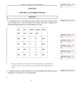
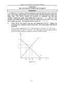
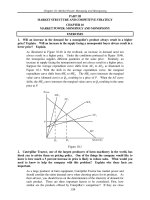
a. Sketch the world demand curve W, the non-OPEC supply curve S, OPEC’s net
demand curve D, and OPEC’s marginal revenue curve. For purposes of
approximation, assume OPEC’s production cost is zero. Indicate OPEC’s optimal
price, OPEC’s optimal production, and non-OPEC production on the diagram.
Now, show on the diagram how the various curves will shift, and how OPEC’s
optimal price will change if non-OPEC supply becomes more expensive because
reserves of oil start running out.
OPEC’s net demand curve, D, is:
DP P=−
−
160 3
1
3
12 12//
.

OPEC’s marginal revenue curve starts from the same point on the vertical axis as
its net demand curve and is twice as steep. OPEC’s optimal production occurs
where MR = 0 (since production cost is assumed to be zero), and OPEC’s optimal
price in Figure 12.12.a.i is found from the net demand curve at Q
OPEC
. Non-
OPEC production can be read off of the non-OPEC supply curve at a price of P*.

Note that in the two figures below, the demand and supply curves are actually non-
linear. They have been drawn in a linear fashion for ease of accuracy.
211
Chapter 12: Monopolistic Competition and Oligopoly
Price
Quantity
MR
D = W - S
S
Q
W
D
W
Q
Non-OPEC
P*
Q
OPEC

Figure 12.12.a.i
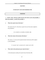
Next, suppose non-OPEC oil becomes more expensive. Then the supply curve S
shifts to S*. This changes OPEC’s net demand curve from D to D*, which in turn
creates a new marginal revenue curve, MR*, and a new optimal OPEC production
level of , yielding a new higher price of P*. At this new price, non-OPEC
production is
Q
D
*
Q
Non OPEC−

*
.
. Notice that the curves must be drawn accurately to give
this result, and again have been drawn in a linear fashion as opposed to non-linear
for ease of accuracy.
Price
Quantity
MR
D = W - S
S
Q
W
D
W
Q
Non-OPEC
P*
Q
OPEC
S*
P**
MR *
D* = W* - S*
Q*
Non-OPEC
Q*
D

Figure 12.12.a.ii
212

Chapter 12: Monopolistic Competition and Oligopoly
b. Calculate OPEC’s optimal (profit-maximizing) price. (Hint: Because OPEC’s cost is
zero, just write the expression for OPEC revenue and find the price that maximizes
it.)
Since costs are zero, OPEC will choose a price that maximizes total revenue:
Max π = PQ = P(W - S)
π
= P 160P
−1/ 2
− 3
1
3
P
1/ 2⎛
⎝
⎞

⎠
=160P
1/2
− 3
1
3
P
3/2
.

To determine the profit-maximizing price, we find the change in the profit function
with respect to a change in price and set it equal to zero:
∂

π
∂P
= 80P
−1/2
− 3
1
3
⎛
⎝
⎞

⎠
3
2
⎛
⎝
⎞

⎠
P
1/2
= 80P
−1/2
− 5P
1/ 2
= 0.

Solving for P,
5P
1

2
=
80
P
1
2
, or P = $16.

c. Suppose the oil-consuming countries were to unite and form a “buyers’ cartel” to
gain monopsony power. What can we say, and what can’t we say, about the impact
this would have on price?
If the oil-consuming countries unite to form a buyers’ cartel, then we have a
monopoly (OPEC) facing a monopsony (the buyers’ cartel). As a result, there is
no well-defined demand or supply curve. We expect that the price will fall below
the monopoly price when the buyers also collude, because monopsony power
offsets monopoly power. However, economic theory cannot determine the exact
price that results from this bilateral monopoly because the price depends on the
bargaining skills of the two parties, as well as on other factors, such as the
elasticities of supply and demand.
13. Suppose the market for tennis shoes has one dominant firm and five fringe firms.
The market demand is Q=400-2P. The dominant firm has a constant marginal cost of 20.
The fringe firms each have a marginal cost of MC=20+5q.
a. Verify that the total supply curve for the five fringe firms is
Q
f
=
P
− 20
.
The total supply curve for the five firms is found by horizontally summing the

five marginal cost curves, or in other words, adding up the quantity supplied by
each firm for any given price. Rewrite the marginal cost curve as follows:
MC
=
20
+
5q
=
P
5q = P − 20
q =
P
5
− 4

Since each firm is identical, the supply curve is five times the supply of one firm
for any given price:
Q
f
= 5(
P
5
− 4)= P − 20
.
213
b. Find the dominant firm’s demand curve.
Chapter 12: Monopolistic Competition and Oligopoly
The dominant firm’s demand curve is given by the difference between the market
demand and the fringe total supply curve:
Q

D
= 400
−
2
P
−
(
P
−
20)
=
420
−
3
P
.
c. Find the profit-maximizing quantity produced and price charged by the dominant
firm, and the quantity produced and price charged by each of the fringe firms.
The dominant firm will set marginal revenue equal to marginal cost. The
marginal revenue curve can be found by recalling that the marginal revenue curve
has twice the slope of the linear demand curve, which is shown below:
Q
D
=
420
−
3P
P = 140−
1
3

Q
D
MR =140−
2
3
Q
D
.

We can now set marginal revenue equal to marginal cost in order to find the
quantity produced by the dominant firm, and the price charged by the dominant
firm:
MR =140−
2
3
Q
D
= 20 = MC

Q
=
180
P
=
80.
Each fringe firm will charge the same price as the dominant firm and the total
output produced by the fringe will be
Q
f
=

P
−
20
=
60.
Each fringe firm will
produce 12 units.

d. Suppose there are ten fringe firms instead of five. How does this change your
results?
We need to find the fringe supply curve, the dominant firm demand curve, and the
dominant firm marginal revenue curve as was done above. The new total fringe
supply curve is
Q
f
= 2
P
− 40.
The new dominant firm demand curve is
Q
D
= 440 − 4
P
.
The new dominant firm marginal revenue curve is
MR =110−
Q
2
.
The dominant firm will produce where marginal revenue is

equal to marginal cost which occurs at 180 units. Substituting a quantity of 180
into the demand curve faced by the dominant firm results in a price of $65.
Substituting the price of $65 into the total fringe supply curve results in a total
fringe quantity supplied of 90, so that each fringe firm will produce 9 units. The
market share of the dominant firm drops from 75% to 67%.
e. Suppose there continue to be five fringe firms but they each manage to reduce their
marginal cost to MC=20+2q. How does this change your results?
Again, we will follow the same method as we did in earlier parts of this problem.
Rewrite the fringe marginal cost curve to get
q =
P
2
−10.
The new total fringe
214
Chapter 12: Monopolistic Competition and Oligopoly
supply curve is five times the individual fringe supply curve, which is just the
marginal cost curve:
Q
f
=
5
2
P − 50.
The new dominant firm demand curve is
found by subtracting the fringe supply curve from the market demand curve to get
Q
D
= 450 − 4.5
P

.
The new dominant firm marginal revenue curve is
MR =100−
2Q
4.5
.
The dominant firm will produce 180 units, price will be $60,
and each fringe firm will produce 20 units. The market share of the dominant
firm drops from 75% to 64%.
14. A lemon-growing cartel consists of four orchards. Their total cost functions are:
TC = 20 + 5Q
11
2

TC = 25 + 3Q
22
2

TC = 15 + 4Q
33
2

TC = 20 + 6Q
44
2

(TC is in hundreds of dollars, Q is in cartons per month picked and shipped.)
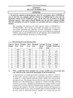
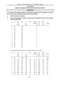
a. Tabulate total, average, and marginal costs for each firm for output levels between 1
and 5 cartons per month (i.e., for 1, 2, 3, 4, and 5 cartons).

The following tables give total, average, and marginal costs for each firm.

Firm 1 Firm 2
Units
TC AC MC TC AC MC
0 20 __ __ 25 __ __
1 25 25 5 28 28 3
2 40 20 15 37 18.5 9
3 65 21.67 25 52 17.3 15
4 100 25 35 73 18.25 21
5 145 29 45 100 20 27

Firm 3 Firm 4
Units
TC AC MC TC AC MC
0 15 __ __ 20 __ __
1 19 19 4 26 26 6
2 31 15.5 12 44 22 18
3 51 17 20 74 24.67 30
4 79 19.75 28 116 29 42
5 115 23 36 170 34 54
215