Tài liệu Bài tập về Kinh tế vĩ mô bằng tiếng Anh - Chương 16 doc

Chapter 16: General Equilibrium and Economic Efficiency
255
PART IV
INFORMATION, MARKET FAILURE,
AND THE ROLE OF GOVERNMENT
CHAPTER 16
GENERAL EQUILIBRIUM AND ECONOMIC EFFICIENCY
EXERCISES
1. Suppose gold (G) and silver (S) are substitutes for each other because both serve as
hedges against inflation. Suppose also that the supplies of both are fixed in the short run
(Q
G
= 75, and Q
S
= 300), and that the demands for gold and silver are given by the
following equations:
P
G
= 975 - Q
G
+ 0.5P
S
and P
S
= 600 - Q
S
+ 0.5P
G
.
a. What are the equilibrium prices of gold and silver?
In the short run, the quantity of gold, Q

G
, is fixed at 75. Substitute Q
G
into the
demand equation for gold:
P
G
= 975 - 75 + 0.5P
S
.
Chapter 16: General Equilibrium and Economic Efficiency
256
In the short run, the quantity of silver, Q
S
, is fixed at 300. Substituting Q
S
into the
demand equation for silver:
P
S
= 600 - 300 + 0.5P
G
.
Since we now have two equations and two unknowns, substitute the price of gold
into the price of silver demand function and solve for the price of silver:
P
S
= 600 - 300 + (0.5)(900 + 0.5P
S
) = $1,000.

Now substitute the price of silver into the demand for gold function:
P
G
= 975 - 75 + (0.5)(1,000) = $1,400.
b. Suppose a new discovery of gold doubles the quantity supplied to 150. How will this
discovery affect the prices of both gold and silver?
When the quantity of gold increases by 75 units from 75 to 150, we must resolve
our system of equations:
P
G
= 975 - 150 + 0.5P
S
, or P
G
= 825 + (0.5)(300 + 0.5P
G
) = $1,300.
The price of silver is equal to:
P
S
= 600 - 300 + (0.5)(1,300) = $950.
2. Using general equilibrium analysis, and taking into account feedback effects, analyze
the following.
Chapter 16: General Equilibrium and Economic Efficiency
257
a. The likely effects of outbreaks of disease on chicken farms on the markets for
chicken and pork.
If consumers are worried about the quality of the chicken then they may choose to
consume pork instead. This will shift the demand curve for pork up and to the
right and the demand curve for chicken down and to the left. The feedback

effects will partially offset these shifts in the two demand curves. As the price
of pork rises, some people may switch back to chicken. This will shift the
demand curve for chicken back to the right by some amount and the demand
curve for pork back to the left by some amount. Overall, we would expect the
price of chicken to be lower and the price of pork higher, but not by as much as if
there were no feedback effects.
b. The effects of increased taxes on airline tickets on travel to major tourist
destinations such as Florida and California, and on the hotel rooms in those
destinations.
Given the increase in the airline tax makes it more costly to travel, the demand
curve for airline tickets will shift down and to the left, reducing the price of
airline tickets. The reduction in the sale of airline tickets will reduce the demand
for hotel rooms by out of town visitors, causing the demand curve for hotel rooms
to shift down and to the left, reducing the price of a hotel room. For the
feedback effects, the lower price for airline tickets and hotel rooms may
encourage some consumers to travel more, in which case both demand curves
shift back up and to the right by some amount, offsetting the initial decline in the
two prices by some amount. We would still expect both prices to be lower, all
else the same.
3. Jane has 3 liters of soft drinks and 9 sandwiches. Bob, on the other hand, has 8 liters of
soft drinks and 4 sandwiches. With these endowments, Jane’s marginal rate of substitution
(MRS) of soft drinks for sandwiches is 4 and Bob’s MRS is equal to 2. Draw an Edgeworth
Chapter 16: General Equilibrium and Economic Efficiency
258
box diagram to show whether this allocation of resources is efficient. If it is, explain why.
If it is not, what exchanges will make both parties better off?
Given that MRS
Bob
≠ MRS
Jane

, the current allocation of resources is inefficient.
Jane and Bob could trade to make one of them better off without making the other
worse off. Although we do not know the exact shape of Jane and Bob’s
indifference curves, we do know the slope of both indifference curves at the current
allocation, because we know that MRS
Jane
= 4 and MRS
Bob
= 2. At the current
allocation point, Jane is willing to trade 4 sandwiches for 1 drink, or she will give
up 1 drink in exchange for 4 sandwiches. Bob is willing to trade 2 sandwiches for
1 drink, or he will give up 1 drink in exchange for 2 sandwiches. Jane will give 4
sandwiches for 1 drink while Bob is willing to accept only 2 sandwiches in
exchange for 1 drink. If Jane gives Bob 3 sandwiches for 1 drink, she is better off
because she was willing to give 4 but only had to give 3. Bob is better off because
he was willing to accept 2 sandwiches and actually received 3. Jane ends up with
4 drinks and 6 sandwiches and Bob ends up with 7 drinks and 7 sandwiches. If
Jane instead was to trade drinks for sandwiches, she would sell a drink for 4
sandwiches. Bob however would not give her more than 2 sandwiches for a drink.
Neither would be willing to make this trade.
4. Jennifer and Drew consume orange juice and coffee. Jennifer’s MRS of orange juice
for coffee is 1 and Drew’s MRS of orange juice for coffee is 3. If the price of orange juice
is $2 and the price of coffee is $3, which market is in excess demand? What do you expect
to happen to the prices of the two goods?
Jennifer is willing to trade 1 coffee for 1 orange juice. Drew is willing to trade 3
coffee for one orange juice. In the market, it is possible to trade 2/3 of a coffee
for an orange juice. Both will find it optimal to trade coffee in exchange for
orange juice since they are willing to give up more for orange juice than they
have to. There is an excess demand of orange juice and an excess supply of
coffee. Price of coffee will go down and price of orange juice will go up.

Chapter 16: General Equilibrium and Economic Efficiency
259
Notice also that at the given rates of MRS and prices, both Jennifer and Drew
have a higher marginal utility per dollar for orange juice as compared to coffee.
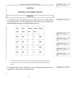
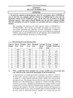
5. Fill in the missing information in the following tables. For each table, use the
information provided to identify a possible trade. Then identify the final allocation and a
possible value for the MRS at the efficient solution. (Note: there is more than one correct
answer.) Illustrate your results using Edgeworth Box diagrams.
a. Norman’s MRS of food for clothing is 1 and Gina’s MRS of food for clothing is 4.

Individual Initial
Allocation
Trade Final
Allocation
Norman 6F,2C 1F for 3C 5F,5C
Gina 1F,8C 3C for 1F 2F,5C

Gina will give 4 clothing for 1 food while Norman is willing to accept only 1
clothing for 1 food. If they settle on 2 or 3 units of clothing for one unit of food
they will both be better off. Let’s say they settle on 3 units of clothing for 1 unit
of food. Gina will give up 3 units of clothing and receive 1 unit of food so her
final allocation is 2F and 5C. Norman will give up 1 food and gain 3 clothing so
his final allocation is 5F and 5C. Gina’s MRS will decrease and Norman’s will
Chapter 16: General Equilibrium and Economic Efficiency
260
increase, so given they must be equal in the end, it will be somewhere between 1
and 4, in absolute value terms.
b. Michael’s MRS of food for clothing is 1/2 and Kelly’s MRS of food for clothing is 3.

Individual Initial

Allocation
Trade Final
Allocation
Michael 10F,3C 1F for 1C 9F,4C
Kelly 5F,15C 1C for 1F 6F,14C

Michael will give 2 food for 1 clothing while Kelly is willing to accept only 1/3
food for 1 clothing. If they settle on 1 unit of food for 1 unit of clothing they
will both be better off. Michael will give up 1 unit of food and receive 1 unit of
clothing so his final allocation is 9F and 4C. Kelly will give up 1 clothing and
gain 1 food so her final allocation is 6F and 14C. Kelly’s MRS will decrease
and Michael’s will increase, so given they must be equal in the end, it will be
somewhere between 3 and 1/2, in absolute value terms.


Chapter 16: General Equilibrium and Economic Efficiency

6. In the analysis of an exchange between two people, suppose both people have identical
preferences. Will the contract curve be a straight line? Explain. Can you think of a
counterexample?
Given that the contract curve intersects the origin for each individual, a straight line
contract curve would be a diagonal line running from one origin to the other. The
slope of this line is
Y
X
, where Y is the total amount of the good on the vertical axis
and X is the total amount of the good on the horizontal axis.
(
are the
amounts of the two goods allocated to one individual and

x
1
,y
1
)
x
2
,y
2
(
)
=
X − x
1
,Y − y
1
()

are the amounts of the two goods allocated to the other individual; the contract
curve may be represented by the equation
1
y
=
Y
X
⎛
⎝
⎞

⎠

1
x .

We need to show that when the marginal rates of substitution for the two
individuals are equal (MRS
1
= MRS
2
), the allocation lies on the contract curve.
For example, consider the utility function . Then
Uxy
ii
=
2
i
MRS =
MU
x
i
MU
y
i
=
2x
i
y
i
x
i
2

=
2y
i
x
i
.

If MRS
1
equals MRS
2
, then
1
2y
1x
⎛
⎝
⎜
⎞

⎠
⎟
=
2
2y
2x
⎛
⎝
⎜
⎞

⎠
⎟
.

261
Chapter 16: General Equilibrium and Economic Efficiency
Is this point on the contract curve? Yes, because
x
2
= X - x
1
and y
2
= Y - y
1
,
2
y
1
x
1
⎛
⎝
⎜
⎞

⎠
⎟
= 2

Y − y
1
X − x
1
⎛
⎝
⎜
⎞

⎠
⎟
.
This means that
y
1
X − x
1
()
x
1
= Y − y
1
, or
y
1
X
−
y
1
x

1
x
1
= Y − y
1
,
and

y
1
X
x
1
− y
1
= Y − y
1
, or
y
1
X
x
1
= Y , or y
1
=
Y
X
⎛
⎝

⎞

⎠
x
1
.

With this utility function we find MRS
1
= MRS
2
, and the contract curve is a straight
line. However, if the two traders have identical preferences but different incomes,
the contract curve is not a straight line when one good is inferior.
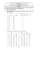
7. Give an example of conditions when the production possibilities frontier might not be
concave.
The production possibilities frontier is concave if at least one of the production
functions exhibits decreasing returns to scale. If both production functions exhibit
constant returns to scale, then the production possibilities frontier is a straight line.
If both production functions exhibit increasing returns to scale, then the production
function is convex. The following numerical examples can be used to illustrate
this concept. Assume that L is the labor input, and X and Y are the two goods.
The first example is the decreasing returns to scale case, the second example is the
262
Chapter 16: General Equilibrium and Economic Efficiency
263
constant returns to scale case, and the third example is the increasing returns to
scale case. Note further that it is not necessary that both products have identical
production functions.
Product X Product Y PPF

L X L Y X Y
0 0 0 0 0 30
1 10 1 10 10 28
2 18 2 18 18 24
3 24 3 24 24 18
4 28 4 28 28 10
5 30 5 30 30 0

Product X Product Y PPF

L X L Y X Y
0 0 0 0 0 50
Chapter 16: General Equilibrium and Economic Efficiency
264
1 10 1 10 10 40
2 20 2 20 20 30
3 30 3 30 30 20
4 40 4 40 40 10
5 50 5 50 50 0

Product X Product Y PPF
L X L Y X Y
0 0 0 0 0 80
1 10 1 10 10 58
2 22 2 22 22 38
3 38 3 38 38 22
4 58 4 58 58 10
5 80 5 80 80 0
Chapter 16: General Equilibrium and Economic Efficiency
265

8. A monopsonist buys labor for less than the competitive wage. What type of inefficiency
will this use of monopsony power cause? How would your answer change if the
monopsonist in the labor market were also a monopolist in the output market?
When market power exists, the market will not allocate resources efficiently. If
the wage paid by a monopsonist is below the competitive wage, too little labor will
be used in the production process. However, output may increase because inputs
are generally less costly. If the firm is a monopolist in the output market, output
will be such that price is above marginal cost and output will clearly be less. With
monopsony, too much may be produced; with monopoly, too little is produced.
The incentive to produce too little could be less than, equal to, or greater than the
incentive to produce too much. Only in a special configuration of marginal
expenditure and marginal revenue would the two incentives be equal.


9. The Acme Corporation produces x and y units of goods Alpha and Beta, respectively.
a. Use a production possibility frontier to explain how the willingness to produce more
or less Alpha depends on the marginal rate of transformation of Alpha or Beta.
The production-possibilities frontier shows all efficient combinations of Alpha and
Beta. The marginal rate of transformation of Alpha for Beta is the slope of the
production-possibilities frontier. The slope measures the marginal cost of
producing one good relative to the marginal cost of producing the other. To
increase x, the units of Alpha, Acme must release inputs in the production of Beta
Chapter 16: General Equilibrium and Economic Efficiency
266
and redirect them to producing Alpha. The rate at which it can efficiently
substitute away from Beta to Alpha is given by the marginal rate of transformation.
b. Consider two cases of production extremes: (i) Acme produces zero units of Alpha
initially, or (ii) Acme produces zero units of Beta initially. If Acme always tries to
stay on its production-possibility frontier, describe the initial positions of cases (i) and

(ii). What happens as the Acme Corporation begins to produce both goods?
The two extremes are corner solutions to the problem of determining efficient
output, given market prices. These two solutions are both possible with different
price ratios, which could produce tangencies with Acme’s end of the frontier.
Assuming that the price ratio changes so the firm would find it efficient to produce
both goods and, assuming the usual concave shape of the frontier, it is likely that the
firm will be able to decrease the production of its primary output by a small amount
for a larger gain in the output of the other good. The firm should continue to shift
production until the ratio of marginal costs (i.e., the MRT) is equal to the ratio of
market prices for the two outputs.
10. In the context of our analysis of the Edgeworth production box, suppose a new invention
causes a constant-returns-to-scale production process for food to become a sharply-
increasing-returns process. How does this change affect the production-contract curve?
In the context of an Edgeworth production box, the production-contract curve is
made up of the points of tangency between the isoquants of the two production
processes. A change from a constant-returns-to-scale production process to a
sharply-increasing-returns-to-scale production process does not necessarily imply a
change in the shape of the isoquants. One can simply redefine the quantities
associated with each isoquant such that proportional increases in inputs yield
greater-than-proportional increases in outputs. Under this assumption, the
marginal rate of technical substitution would not change. Thus, there would be no
change in the production-contract curve.
Chapter 16: General Equilibrium and Economic Efficiency
If, however, accompanying this change to a sharply-increasing-returns-to-scale
technology, there were a change in the trade-off between the two inputs (a change in
the shape of the isoquants), then the production-contract curve would change. For
example, if the original production function were Q = LK with
MRTS
L
=

K
, the
shape of the isoquants would not change if the new production function were Q =
L
2
K
2
with
MRTS
L
=
K
K
, but the shape would change if the new production function
were Q = L
2
K with
MRTS= 2
L
⎛
⎝
⎞

⎠

. Note that in this case the production
possibilities frontier is likely to become convex.

267
Chapter 16: General Equilibrium and Economic Efficiency

268
11. Suppose that country A and country B both produce wine and cheese. Country A
has 800 units of available labor, while country B has 600 units. Prior to trade, country A
consumes 40 pounds of cheese and 8 bottles of wine, and country B consumes 30 pounds of
cheese and 10 bottles of wine.

Country A Country B
labor per pound cheese 10 10
labor per bottle wine 50 30

a. Which country has a comparative advantage in the production of each good?
Explain.
To produce another bottle of wine, Country A needs 50 units of labor, and must therefore
produce five fewer units of cheese. The opportunity cost of a bottle of wine is five
pounds of cheese. For Country B the opportunity cost of a bottle of wine is three
pounds of cheese. Since Country B has a lower opportunity cost, they should produce
the wine and Country A should produce the cheese. The opportunity cost of cheese in
Country A is 1/5 of a bottle of wine and in Country B is 1/3 of a bottle of wine.
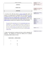
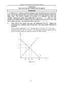
b. Determine the production possibilities curve for each country, both graphically and
algebraically. (Label the pre-trade production point PT and the post trade
production point P.)
Chapter 16: General Equilibrium and Economic Efficiency
For Country A their production frontier is given by 10C+50W=800, or C=80-5W, and for
Country B their production frontier is given by 10C+30W=600, or C=60-3W. The
slope of the frontier for Country A is -5 which is the price of wine divided by the price of
cheese. Therefore, in Country A the price of wine is 5 and in Country B the price of
wine is 3. After trade, the price will settle in the middle somewhere. The post trade
production point is on the terms of trade line which has a slope equal to the world price
ratio, say –4 in this case. Country A will produce only cheese and Country B will
produce only wine. Each can consume at a point on the terms of trade line that lies

above and outside the production frontier.
C
W
16
80
C
P
PT

Country A
c. Given that 36 pounds of cheese and 9 bottles of wine are traded, label the post trade
consumption point C.
See the graph for Country A above. Before trade the country consumed and
produced at point PT, which was given as 40 pounds of cheese and 8 bottles of
wine. After trade, Country A will completely specialize in the production of
cheese and will produce at point P. Given the quantities traded, Country A will
consume 80-36=44 pounds of cheese and 0+9 bottles of wine. This is point C on
the graph. The graph for Country B is similar except that Country B will
produce only wine and the trade line will intersect their production frontier on the
wine axis.
269
Chapter 16: General Equilibrium and Economic Efficiency
270

d. Prove that both countries have gained from trade?
Both countries have gained from trade because they can now both consume more of both
goods that they could before trade. Graphically we can see this by noticing that the
trade line lies to the left of the production frontier. After trade, the country can consume
on the trade line and is able to consume more of both goods. Numerically, Country A
consumes 4 more pounds of cheese and 1 more bottle of wine after trade as compared to

pre-trade, and Country B consumes 6 more pounds of cheese and 1 more bottle of wine.
e. What is the slope of the price line at which trade occurs?
We assumed –4, which is somewhere between the pre-trade prices. All that we
can say from the information given is that it will be somewhere between the pre-
trade prices, or the slopes of the two production frontiers. We would need more
information about demand for the two products in each country to determine the
exact post-trade prices.