Tài liệu Advanced DSP and Noise reduction P7 docx
Bạn đang xem bản rút gọn của tài liệu. Xem và tải ngay bản đầy đủ của tài liệu tại đây (135.92 KB, 22 trang )
7
ADAPTIVE FILTERS
7.1 State-Space Kalman Filters
7.2 Sample-Adaptive Filters
7.3 Recursive Least Square (RLS) Adaptive Filters
7.4 The Steepest-Descent Method
7.5 The LMS Filter
7.6 Summary
daptive filters are used for non-stationary signals and
environments, or in applications where a sample-by-sample
adaptation of a process or a low processing delay is required.
Applications of adaptive filters include multichannel noise reduction,
radar/sonar signal processing, channel equalization for cellular mobile
phones, echo cancellation, and low delay speech coding. This chapter
begins with a study of the state-space Kalman filter. In Kalman theory a
state equation models the dynamics of the signal generation process, and an
observation equation models the channel distortion and additive noise.
Then we consider recursive least square (RLS) error adaptive filters. The
RLS filter is a sample-adaptive formulation of the Wiener filter, and for
stationary signals should converge to the same solution as the Wiener filter.
In least square error filtering, an alternative to using a Wiener-type closed-
form solution is an iterative gradient-based search for the optimal filter
coefficients. The steepest-descent search is a gradient-based method for
searching the least square error performance curve for the minimum error
filter coefficients. We study the steepest-descent method, and then consider
the computationally inexpensive LMS gradient search method.
A
z
–1
w
k
(
m+
1)
α
y
(
m
)
e
(
m
)
µ
α
w
(
m
)
Advanced Digital Signal Processing and Noise Reduction, Second Edition.
Saeed V. Vaseghi
Copyright © 2000 John Wiley & Sons Ltd
ISBNs: 0-471-62692-9 (Hardback): 0-470-84162-1 (Electronic)
206
Adaptive Filters
7.1 State-Space Kalman Filters
The Kalman filter is a recursive least square error method for estimation of
a signal distorted in transmission through a channel and observed in noise.
Kalman filters can be used with time-varying as well as time-invariant
processes. Kalman filter theory is based on a state-space approach in which
a state equation models the dynamics of the signal process and an
observation equation models the noisy observation signal. For a signal x(m)
and noisy observation y(m), the state equation model and the observation
model are defined as
)()1()1,()(
mmmmm
exx
+−−=
Φ
(7.1)
)()()()(
mmmm
nx
y
+=
Η
(7.2)
where
x(m) is the P-dimensional signal, or the state parameter, vector at time m,
Φ
(m, m–1) is a
P
×
P
dimensional state transition matrix that relates the
states of the process at times m–1 and m,
e(m) is the P-dimensional uncorrelated input excitation vector of the state
equation,
Σ
ee
(m) is the
P
×
P
covariance matrix of e(m),
y(m) is the M-dimensional noisy and distorted observation vector,
H(m) is the
M
×
P
channel distortion matrix,
n(m) is the M-dimensional additive noise process,
Σ
nn
(m) is the
M
×
M
covariance matrix of n(m).
The Kalman filter can be derived as a recursive minimum mean square
error predictor of a signal x(m), given an observation signal y(m). The filter
derivation assumes that the state transition matrix
Φ
(m, m–1), the channel
distortion matrix H(m), the covariance matrix
Σ
ee
(m) of the state equation
input and the covariance matrix
Σ
nn
(m) of the additive noise are given.
In this chapter, we use the notation
()
imm
−
y
ˆ
to denote a prediction of
y(m) based on the observation samples up to the time m–i. Now assume that
()
1
ˆ
−
mm
y
is the least square error prediction of y(m) based on the
observations [y(0), , y(m–1)]. Define a so-called innovation, or prediction
error signal as
()
1
ˆ
)()( −−=
mmmm
y
y
v
(7.3)
State-Space Kalman Filters
207
The innovation signal vector v(m) contains all that is unpredictable from the
past observations, including both the noise and the unpredictable part of the
signal. For an optimal linear least mean square error estimate, the
innovation signal must be uncorrelated and orthogonal to the past
observation vectors; hence we have
[]
0)()(
T
=−
kmm
y
v
E
, k > 0 (7.4)
and
[]
0)()(
T
=
km
vv
E
,
km
≠
(7.5)
The concept of innovations is central to the derivation of the Kalman filter.
The least square error criterion is satisfied if the estimation error is
orthogonal to the past samples. In the following derivation of the Kalman
filter, the orthogonality condition of Equation (7.4) is used as the starting
point to derive an optimal linear filter whose innovations are orthogonal to
the past observations.
Substituting the observation Equation (7.2) in Equation (7.3) and using
the relation
()
[]
()
1
ˆ
)(
1
ˆ
)()1|(
ˆ
−=
−=−
mmm
mmmmm
xH
x
y
y
E
(7.6)
yields
()
)()(
~
)(
1
ˆ
)()()()()(
mmm
mmmmmmm
nxH
xHnxHv
+=
−−+=
(7.7)
where
˜
x
(
m
)
is the signal prediction error vector defined as
()
1
ˆ
)()(
~
−−=
mmmm
xxx
(7.8)
x
(
m
)
e
(
m
)
H
(
m
)
n
(
m
)
y
(
m
)
Z
-1
Φ
(
m,m
-1)
+
+
Figure 7.1
Illustration of signal and observation models in Kalman filter theory.
208
Adaptive Filters
From Equation (7.7) the covariance matrix of the innovation signal is given
by
[]
)()()()(
)()()(
T
~~
T
mmmm
mmm
nnxx
vv
HH
vv
ΣΣ
Σ
+=
=
E
(7.9)
where
Σ
˜
x
˜
x
(m)
is the covariance matrix of the prediction error
˜
x
(m)
. Let
ˆ
x
m+1 m
()
denote the least square error prediction of the signal
x
(
m
+1).
Now, the prediction of
x
(
m
+1), based on the samples available up to the
time
m
, can be expressed recursively as a linear combination of the
prediction based on the samples available up to the time
m–
1 and the
innovation signal at time
m
as
()()
)()(11
ˆ
1
ˆ
mmmmmm
vKx=x
+−++
(7.10)
where the
P
×
M
matrix
K
(
m
)
is the Kalman gain matrix. Now, from
Equation (7.1), we have
() ()
1
ˆ
),1(11
ˆ
−+=−+
mmmmmm
xx
Φ
(7.11)
Substituting Equation (7.11) in (7.10) gives a recursive prediction equation
as
() ()
)()(1
ˆ
),1(1
ˆ
mmmmmmmm
vKx=x
+−++
Φ
(7.12)
To obtain a recursive relation for the computation and update of the
Kalman gain matrix, we multiply both sides of Equation (7.12) by
v
T
(m)
and take the expectation of the results to yield
()
[]
()
[][]
)()()()(1
ˆ
),1()(1
ˆ
TTT
mmmmmmmmmmm
vvK+vxvx
EEE
−+=+
Φ
(7.13)
Owing to the required orthogonality of the innovation sequence and the past
samples, we have
()
[
]
0)(1
ˆ
T
=−
mmm
vx
E
(7.14)
Hence, from Equations (7.13) and (7.14), the Kalman gain matrix is given
by
()
[]
)()(1
ˆ
)(
1T
mmmmm
−
+=
vv
vxK
Σ
E
(7.15)
State-Space Kalman Filters
209
The first term on the right-hand side of Equation (7.15) can be expressed as
()
[]
()
()()
[]
()
[]
()
()()
[]
()()()
[]
()()
[]
()()
[]
)(1
~
1
~
),1(
)(1
~
)(1
~
1
ˆ
),1(
1
ˆ
)()1()(),1(
)(1
)(1
~
1)(1
ˆ
TT
T
T
T
TT
mmmmmmm
mmmmmmmmmm
mmmmmmm
mm
mmmmmmm
Hxx
nxHxx
yyex
vx
vxxvx
−−+=
+−−+−+=
−−+++=
+=
+−+=+
E
E
E
E
EE
Φ
Φ
Φ
(7.16)
In developing the successive lines of Equation (7.16), we have used the
following relations:
()
[]
0)(|1
~
T
=+
mmm
vx
E
(7.17)
()()
[
]
01|
ˆ
)()1(
T
=−−+
mmmm
yye
E
(7.18)
x
(
m
)
=
ˆ
x
(
m
|
m
−
1)
+
˜
x
m
|
m
−
1
()
(7.19)
()
[]
01|
~
)1|(
ˆ
=−−
mmmm
xx
E
(7.20)
and we have also used the assumption that the signal and the noise are
uncorrelated. Substitution of Equations (7.9) and (7.16) in Equation (7.15)
yields the following equation for the Kalman gain matrix:
()
[]
1
T
~~
T
~~
)()()()()()(),1(
−
++=
mmmmmmmmm
nnxxxx
HHHK
ΣΣΣΦ
(7.21)
where
Σ
˜
x
˜
x
(
m
)
is the covariance matrix of the signal prediction error
˜
x
(
m
|
m
−
1)
. To derive a recursive relation for
Σ
˜
x
˜
x
(
m
)
, we consider
()
()
()
1
ˆ
1
~
−−=−
mmmmm
xxx
(7.22)
Substitution of Equation (7.1) and (7.12) in Equation (7.22) and
rearrangement of the terms yields
()
[]
()
[]
()
[]
()
)1()1()(1
~
)1()1()1,(
)1()1()1(
~
)1()1()(1
~
)1,(
)1()1(21
ˆ
)1,()()1()1,(1|
~
−−−−−−−=
−−−−−−−−=
−−−−−−−−=−
mm+mmmmmm
mm+mmmmmmm
mmmmmmmmmmmm
nKe+xHK
nKxHKe+x
vK+xe+xx
Φ
Φ
ΦΦ
(7.23)
210
Adaptive Filters
From Equation (7.23) we can derive the following recursive relation for the
variance of the signal prediction error
)1()1()1()()(1)()()(
TT
~~~~
−−−++−= mmmmmmmm KKLL
nneexxxx
ΣΣΣΣ
(7.24)
where the
P
×
P
matrix
L
(
m
) is defined as
[]
)1()1()1,()( −−−−= mmmmm HKL
Φ
(7.25)
Kalman Filtering Algorithm
Input: observation vectors {
y
(
m
)}
Output: state or signal vectors {
ˆ x
(m)
}
Initial conditions:
I
δ
=(0)
~~
xx
Σ
(7.26)
()
010
ˆ
=−x
(7.27)
For
m
= 0, 1,
Innovation signal:
v(m)
=
y(m )
−
H(m)
ˆ
x (m|m
−
1)
(7.28)
Kalman gain:
[]
1
T
~~
T
~~
)()()()()()(),1()(
−
++= mmmmmmmmm
nnxxxx
HHHK
ΣΣΣΦ
(7.29)
Prediction update:
ˆ
x m
+
1| m
()
=
Φ
(m
+
1, m)
ˆ
x m|m
−
1
()
+
K(m)v(m)
(7.30)
Prediction error correlation matrix update:
L
(m+1)
=
Φ
(m
+
1, m)
−
K
(m)
H
(m)
[]
(7.31)
)()()()1()1()()1(1)(
T
~~~~
mmmmmmmm KKLL
nneexxxx
ΣΣΣΣ
+++++=+
(7.32)
Example 7.1
Consider the Kalman filtering of a first-order AR process
x
(
m
) observed in an additive white Gaussian noise
n
(
m
). Assume that the
signal generation and the observation equations are given as
x
(
m
)
=
a
(
m
)
x
(
m
−
1)
+
e
(
m
)
(7.33)
State-Space Kalman Filters
211
y
(
m
)
=
x
(
m
)
+
n
(
m
)
(7.34)
Let
σ
e
2
(
m
)
and
σ
n
2
(
m
)
denote the variances of the excitation signal e(m)
and the noise n(m) respectively. Substituting
Φ
(m+1,m)=a(m) and H(m)=1
in the Kalman filter equations yields the following Kalman filter algorithm:
Initial conditions:
δσ
=
x
(0)
2
~
(7.35)
()
010
ˆ
=x
−
(7.36)
For m = 0, 1,
Kalman gain:
)()(
)()1(
)(
22
~
2
~
mm
mma
mk
nx
x
σσ
σ
+
+
=
(7.37)
Innovation signal:
v(m)
=
y
(
m
)
−
ˆ
x m | m
−
1
() (7.38)
Prediction signal update:
ˆ
x
(
m
+
1|
m
)
=
a
(
m
+
1)
ˆ
x
(
m
|
m
−
1)
+
k
(
m
)
v
(
m
)
(7.39)
Prediction error update:
σ
˜
x
2
(m
+
1)
=
a
(
m
+
1)
−
k
(
m
)
[]
2
σ
˜
x
2
(m)
+
σ
e
2
(
m
+
1)
+
k
2
(
m
)
σ
n
2
(
m
)
(7.40)
where
σ
˜
x
2
(m)
is the variance of the prediction error signal.
Example 7.2
Recursive estimation of a constant signal observed in noise.
Consider the estimation of a constant signal observed in a random noise.
The state and observation equations for this problem are given by
x
(
m
)
=
x
(
m
−
1)
=
x
(7.41)
y
(
m
)
=
x
+
n
(
m
)
(7.42)
Note that
Φ
(m,m–1)=1, state excitation e(m)=0 and H(m)=1. Using the
Kalman algorithm, we have the following recursive solutions:
Initial Conditions:
σ
˜
x
2
(0)
=
δ
(7.43)
ˆ
x
0
−
1
()
=
0
(7.44)
212
Adaptive Filters
For m = 0, 1,
Kalman gain:
)()(
)(
)(
22
~
2
~
mm
m
mk
nx
x
σσ
σ
+
=
(7.45)
Innovation signal:
()
1
ˆ
)()(
−−=
m|mxmymv
(7.46)
Prediction signal update:
)()()1|(
ˆ
)|1(
ˆ
mvmkmmxmmx
+−=+
(7.47)
Prediction error update:
[]
)()()()(11)
222
~
2
2
~
mmkmmk+(m
nxx
σσσ
+−=
(7.48)
7.2 Sample-Adaptive Filters
Sample adaptive filters, namely the RLS, the steepest descent and the LMS,
are recursive formulations of the least square error Wiener filter. Sample-
adaptive filters have a number of advantages over the block-adaptive filters
of Chapter 6, including lower processing delay and better tracking of non-
stationary signals. These are essential characteristics in applications such as
echo cancellation, adaptive delay estimation, low-delay predictive coding,
noise cancellation, radar, and channel equalisation in mobile telephony,
where low delay and fast tracking of time-varying processes and
environments are important objectives.
Figure 7.2 illustrates the configuration of a least square error adaptive
filter. At each sampling time, an adaptation algorithm adjusts the filter
coefficients to minimise the difference between the filter output and a
desired, or target, signal. An adaptive filter starts at some initial state, and
then the filter coefficients are periodically updated, usually on a sample-by-
sample basis, to minimise the difference between the filter output and a
desired or target signal. The adaptation formula has the general recursive
form:
next parameter estimate = previous parameter estimate + update(error)
where the update term is a function of the error signal. In adaptive filtering a
number of decisions has to be made concerning the filter model and the
adaptation algorithm:
Recursive Least Square (RLS) Adaptive Filters
213
(a) Filter type: This can be a finite impulse response (FIR) filter, or an
infinite impulse response (IIR) filter. In this chapter we only consider
FIR filters, since they have good stability and convergence properties
and for this reason are the type most often used in practice.
(b) Filter order: Often the correct number of filter taps is unknown. The
filter order is either set using a priori knowledge of the input and the
desired signals, or it may be obtained by monitoring the changes in the
error signal as a function of the increasing filter order.
(c) Adaptation algorithm: The two most widely used adaptation algorithms
are the recursive least square (RLS) error and the least mean square
error (LMS) methods. The factors that influence the choice of the
adaptation algorithm are the computational complexity, the speed of
convergence to optimal operating condition, the minimum error at
convergence, the numerical stability and the robustness of the algorithm
to initial parameter states.
7.3 Recursive Least Square (RLS) Adaptive Filters
The recursive least square error (RLS) filter is a sample-adaptive, time-
update, version of the Wiener filter studied in Chapter 6. For stationary
signals, the RLS filter converges to the same optimal filter coefficients as
the Wiener filter. For non-stationary signals, the RLS filter tracks the time
variations of the process. The RLS filter has a relatively fast rate of
convergence to the optimal filter coefficients. This is useful in applications
such as speech enhancement, channel equalization, echo cancellation and
radar where the filter should be able to track relatively fast changes in the
signal process.
In the recursive least square algorithm, the adaptation starts with some
initial filter state, and successive samples of the input signals are used to
adapt the filter coefficients. Figure 7.2 illustrates the configuration of an
adaptive filter where y(m), x(m) and w(m)=[w
0
(m), w
1
(m), , w
P–1
(m)]
denote the filter input, the desired signal and the filter coefficient vector
respectively. The filter output can be expressed as
)()()(
ˆ
T
mmmx
y
w
=
(7.49)
214
Adaptive Filters
where
ˆ
x
(
m
)
is an estimate of the desired signal x(m). The filter error signal
is defined as
)()()(
)(
ˆ
)()(
T
mmmx
mxmxme
yw−=
−=
(7.50)
The adaptation process is based on the minimization of the mean square
error criterion defined as
[]
)()()()()(2)0(
)(])()([)()]()([)(2)]([
)()()()]([
TT
TTT2
2
T2
mmmmmr
mmmmmxmmmx
mmmxme
xx
wRwrw
wyywyw
yw
yyyx
+−=
+−=
−=
EEE
EE
(7.51)
The Wiener filter is obtained by minimising the mean square error with
respect to the filter coefficients. For stationary signals, the result of this
minimisation is given in Chapter 6, Equation (6.10), as
yxyy
r Rw
1
−
= (7.52)
Adaptation
algorithm
“Desired” or “target ”
signal
x
(
m
)
Input
y
(
m
)
z
–
1
. . .
y
(
m
–1)
y
(
m
-
P
-1)
x
(
m
)
^
w
1
w
0
Transversal
filter
w
2
y
(
m–2
)
e
(
m
)
z
–1
z
–1
w
P
–1
Figure 7.2
Illustration of the configuration of an adaptive filter.
Recursive Least Square (RLS) Adaptive Filters
215
where R
yy
is the autocorrelation matrix of the input signal and r
yx
is the
cross-correlation vector of the input and the target signals. In the following,
we formulate a recursive, time-update, adaptive formulation of Equation
(7.52). From Section 6.2, for a block of N sample vectors, the correlation
matrix can be written as
∑
−
=
==
1
0
TT
)()(
N
m
mm
y
y
YYR
yy
(7.53)
where y(m)=[y(m), , y(m–P)]
T
. Now, the sum of vector product in
Equation (7.53) can be expressed in recursive fashion as
)()()1()(
T
mmmm
y
y
RR
yy
yy
+−=
(7.54)
To introduce adaptability to the time variations of the signal statistics, the
autocorrelation estimate in Equation (7.54) can be windowed by an
exponentially decaying window:
)()()1()(
T
mmmm
y
y
RR
yy
yy
+−=
λ
(7.55)
where
λ
is the so-called adaptation, or forgetting factor, and is in the range
0>
λ
>1. Similarly, the cross-correlation vector is given by
∑
−
=
=
1
0
)()(
N
m
x
mxm
y
r
y
(7.56)
The sum of products in Equation (7.56) can be calculated in recursive form
as
r
y
x
(
m
)
=
r
y
x
(
m
−
1)
+
y
(
m
)
x
(
m
)
(7.57)
Again this equation can be made adaptive using an exponentially decaying
forgetting factor
λ
:
)()()1()(
mxmmm
yrr
yy
+−=
xx
λ
(7.58)
For a recursive solution of the least square error Equation (7.58), we need to
obtain a recursive time-update formula for the inverse matrix in the form
216
Adaptive Filters
)()1()(
11
mUpdatemm +−=
−−
yyyy
RR
(7.59)
A recursive relation for the matrix inversion is obtained using the following
lemma.
The Matrix Inversion Lemma
Let
A
and
B
be two positive-definite
P
×
P
matrices related by
T11
CCDBA
−−
+=
(7.60)
where
D
is a positive-definite
N
×
N
matrix and
C
is a
P
×
N
matrix. The
matrix inversion lemma states that the inverse of the matrix
A
can be
expressed as
()
BCBCC+DBCBA
T
1
T1
−
−
−=
(7.61)
This lemma can be proved by multiplying Equation (7.60) and Equation
(7.61). The left and right hand sides of the results of multiplication are the
identity matrix. The matrix inversion lemma can be used to obtain a
recursive implementation for the inverse of the correlation matrix
R
y
y
−
1
(
m
)
.
Let
AR
yy
=)(m
(7.62)
BR
yy
=−
−−
)1(
11
m
λ
(7.63)
y
(
m
)
=
C
(7.64)
D
= identity matrix
(7.65)
Substituting Equations (7.62) and (7.63) in Equation (7.61), we obtain
)()1()(1
)1()()()1(
)1()(
1T1
1T12
111
mmm
mmmm
mm
yRy
RyyR
RR
yy
yyyy
yyyy
−+
−−
−−=
−−
−−−
−−−
λ
λ
λ
(7.66)
Now define the variables
Φ
(
m
) and
k
(
m
) as
Φ
yy
(m)
=
R
yy
−
1
(m)
(7.67)
Recursive Least Square (RLS) Adaptive Filters
217
and
)()1()(1
)()1(
)(
1T1
11
mmm
mm
m
yRy
yR
k
yy
yy
−+
−
=
−−
−−
λ
λ
(7.68)
or
)()1()(1
)()1(
)(
T1
1
mmm
mm
m
yy
y
k
yy
yy
−+
−
=
−
−
Φ
Φ
λ
λ
(7.69)
Using Equations (7.67) and (7.69), the recursive equation (7.66) for
computing the inverse matrix can be written as
)1()()()1()(
T11
−−−=
−−
mmmmm
yyyyyy
yk
ΦΦΦ λλ
(7.70)
From Equations (7.69) and (7.70), we have
[]
)()(
)()1()()()1()(
T11
mm
mmmmmm
y
yykk
yy
yyyy
Φ
ΦΦ
=
−−−=
−−
λλ
(7.71)
Now Equations (7.70) and (7.71) are used in the following to derive the
RLS adaptation algorithm.
Recursive Time-update of Filter Coefficients
The least square error
filter coefficients are
)()(
)()( )(
1
mm
mmm
yxyy
yxyy
r
r Rw
Φ
=
=
−
(7.72)
Substituting the recursive form of the correlation vector in Equation (7.72)
yields
w
(m)
=
Φ
yy
(m)
λ
r
yx
(m
−
1)
+
y
(m)x(m)
[]
=
λΦΦ
yy
(m)
r
yx
(m
−
1)
+
Φ
yy
(m)
y
(m)x(m)
(7.73)
Now substitution of the recursive form of the matrix
Φ
yy
(
m
) from Equation
(7.70) and
k
(
m
)
=
Φ
(
m
)
y
(
m
) from Equation (7.71) in the right-hand side of
Equation (7.73) yields
218
Adaptive Filters
[]
)()()1()1()()()1()(
T11
mxmmmmmmm krykw
yxyyyy
+−−−−=
−−
λλλΦΦΦ
(7.74)
or
)()()1()1()()()1()1()(
T
mxmmmmmmmm
krykrw
yxyyyxyy
+−−−−−=
ΦΦ
(7.75)
Substitution of
w
(
m
–1)
=
Φ
(m
–1)
r
yx
(
m
–1) in Equation (7.75) yields
[]
)1()()()()1()(
T
−−−−=
mmmxmmm wykww
(7.76)
This equation can be rewritten in the following form
w
(
m
)
=
w
(
m
−
1)
−
k
(
m
)
e
(
m
)
(7.77)
Equation (7.77) is a recursive time-update implementation of the least
square error Wiener filter.
RLS Adaptation Algorithm
Input signals:
y
(
m
) and
x
(
m
)
Initial values:
I
δ=
)(
m
yy
Φ
I
)0(
ww
=
For
m
= 1,2,
Filter gain vector:
)()1()(1
)()1(
)(
T1
1
mmm
mm
m
yy
y
k
yy
yy
−+
−
=
−
−
Φ
Φ
λ
λ
(7.78)
Error signal equation:
)()1()()(
T
mmmxme yw
−−=
(7.79)
Filter coefficients:
w
(
m
)
=
w
(
m
−
1)
−
k
(
m
)
e
(
m
)
(7.80)
Inverse correlation matrix update:
Φ
yy
(
m
)
=
λ
−
1
Φ
yy
(
m
−
1)
−
λ
−
1
k
(
m
)
y
T
(
m
)
Φ
yy
(
m
−
1)
(7.81)
The Steepest-Descent Method
219
7.4 The Steepest-Descent Method
The mean square error surface with respect to the coefficients of an FIR
filter, is a quadratic bowl-shaped curve, with a single global minimum that
corresponds to the LSE filter coefficients. Figure 7.3 illustrates the mean
square error curve for a single coefficient filter. This figure also illustrates
the steepest-descent search for the minimum mean square error coefficient.
The search is based on taking a number of successive downward steps in
the direction of negative gradient of the error surface. Starting with a set of
initial values, the filter coefficients are successively updated in the
downward direction, until the minimum point, at which the gradient is zero,
is reached. The steepest-descent adaptation method can be expressed as
−+=+
)(
)]([
)()1(
2
m
me
mm
w
ww
∂
∂
µ
E
(7.82)
where
µ
is the adaptation step size. From Equation (5.7), the gradient of the
mean square error function is given by
w(i –2)
w(i–1)
w(i)
w
optimal
E
[e
2
(m)]
w
Figure 7.3
Illustration of gradient search of the mean square error surface for the
minimum error point.
220
Adaptive Filters
)(22
)(
)]([
2
m
m
me
x
wRr
w
yyy
+−=
∂
∂
E
(7.83)
Substituting Equation (7.83) in Equation (7.82) yields
[
]
)()()1( mmm
x
wRrww
yyy
−+=+
µ
(7.84)
where the factor of 2 in Equation (7.83) has been absorbed in the adaptation
step size
µ
. Let
w
o
denote the optimal LSE filter coefficient vector, we
define a filter coefficients error vector
˜ w (
m
)
as
o
www −= )()(
~
mm
(7.85)
For a stationary process, the optimal LSE filter
w
o
is obtained from the
Wiener filter, Equation (5.10), as
x
yyyo
rRw
1
−
= (7.86)
Subtracting
w
o
from both sides of Equation (7.84), and then substituting
R
yy
w
o
for
r
y
x
, and using Equation (7.85) yields
[
]
)(
~
)1(
~
mm wRw
yy
µ
−=+ I
(7.87)
It is desirable that the filter error vector
˜ w
(m)
vanishes as rapidly as
possible. The parameter
µ
, the adaptation step size, controls the stability
and the rate of convergence of the adaptive filter. Too large a value for
µ
causes instability; too small a value gives a low convergence rate. The
stability of the parameter estimation method depends on the choice of the
adaptation parameter
µ
and the autocorrelation matrix. From Equation
(7.87), a recursive equation for the error in each individual filter coefficient
can be obtained as follows. The correlation matrix can be expressed in
terms of the matrices of eigenvectors and eigenvalues as
T
QQ=R
yy
Λ
(7.88)
The Steepest-Descent Method
221
where Q is an orthonormal matrix of the eigenvectors of R
yy
, and
Λ
is a
diagonal matrix with its diagonal elements corresponding to the
eigenvalues of R
yy
. Substituting R
yy
from Equation (7.88) in Equation
(7.87) yields
[]
)(
~
)1(
~
T
mm
w
Q
Q
w
Λ
µ
−=+ I
(7.89)
Multiplying both sides of Equation (7.89) by Q
T
and using the relation
Q
T
Q=QQ
T
=
I
yields
)(
~
][)1(
~
TT
mm
w
Q
w
Q
Λµ
−=+ I
(7.90)
Let
)(
~
)(
T
m=m
w
Q
v
(7.91)
Then
v
(
m+
1)
=
I
−
µΛΛ
[] v
(
m
)
(7.92)
As
Λ
and Ι
are both diagonal matrices, Equation (7.92) can be expressed in
terms of the equations for the individual elements of the error vector v(m)
as
[]
)(11)(
mv=+mv
kkk
λ−
µ
(7.93)
where
λ
k
is the k
th
eigenvalue of the autocorrelation matrix of the filter
input y(m). Figure 7.4 is a feedback network model of the time variations of
the error vector. From Equation (7.93), the condition for the stability of the
adaptation process and the decay of the coefficient error vector is
−
1
<
1
−
µλ
k
<
1
(7.94)
1
–
µλ
k
z
–1
v
k
(
m+
1)
v
k
(
m
)
Figure 7.4
A feedback model of the variation of coefficient error with time.
222
Adaptive Filters
Let
λ
max
denote the maximum eigenvalue of the autocorrelation matrix of
y(m) then, from Equation (7.94) the limits on
µ
for stable adaptation are
given by
0
<
µ
<
2
λ
max
(7.95)
Convergence Rate
The convergence rate of the filter coefficients
depends on the choice of the adaptation step size
µ
, where 0<
µ
<1/
λ
max
.
When the eigenvalues of the correlation matrix are unevenly spread, the
filter coefficients converge at different speeds: the smaller the k
th
eigenvalue the slower the speed of convergence of the k
th
coefficients. The
filter coefficients with maximum and minimum eigenvalues,
λ
max
and
λ
min
converge according to the following equations:
()
)(11)(
maxmaxmax
mv=+mv
λ
µ
−
(7.96)
()
)(11)+(
minminmin
mv=mv
λ
µ
−
(7.97)
The ratio of the maximum to the minimum eigenvalue of a correlation
matrix is called the eigenvalue spread of the correlation matrix:
min
max
spreadeigenvalue
λ
λ
=
(7.98)
Note that the spread in the speed of convergence of filter coefficients is
proportional to the spread in eigenvalue of the autocorrelation matrix of the
input signal.
7.5 The LMS Filter
The steepest-descent method employs the gradient of the averaged squared
error to search for the least square error filter coefficients. A
computationally simpler version of the gradient search method is the least
mean square (LMS) filter, in which the gradient of the mean square error is
substituted with the gradient of the instantaneous squared error function.
The LMS adaptation method is defined as
The LMS Filter
223
−+=+
)(
)(
)()1(
2
m
me
mm
w
ww
∂
∂
µ
(7.99)
where the error signal
e
(
m
) is given by
)()()()(
T
mmmxme xw−=
(7.100)
The instantaneous gradient of the squared error can be re-expressed as
)()(2
)]()()([)(2
)]()()([
)()(
)(
2T
2T
2
mem
mmmxm
mmmx
mm
me
y
ywy
yw
w
=
w
−=
−−=
−
∂
∂
∂
∂
(7.101)
Substituting Equation (7.101) into the recursion update equation of the filter
parameters, Equation (7.99) yields the LMS adaptation equation:
[]
)()()()1( memmm yww
µ
+=+
(7.102)
It can seen that the filter update equation is very simple. The LMS filter is
widely used in adaptive filter applications such as adaptive equalisation,
echo cancellation etc. The main advantage of the LMS algorithm is its
simplicity both in terms of the memory requirement and the computational
complexity which is
O
(
P
), where
P
is the filter length.
z
–1
w
k
(
m+
1)
α
y
(
m
)
e
(
m
)
µ
α
w
(
m
)
Figure 7.5
Illustration of LMS adaptation of a filter coefficient.
224
Adaptive Filters
Leaky LMS Algorithm
The stability and the adaptability of the recursive
LMS adaptation Equation (7.86) can improved by introducing a so-called
leakage factor
α
as
[]
)()()()1( memmm yww
µ
α
+=+
(7.103)
Note that the feedback equation for the time update of the filter coefficients
is essentially a recursive (infinite impulse response) system with input
µ
y
(
m
)
e
(
m
) and its poles at
α
. When the parameter
α
<
1, the effect is to
introduce more stability and accelerate the filter adaptation to the changes
in input signal characteristics.
Steady-State Error:
The optimal least mean square error (LSE),
E
min
, is
achieved when the filter coefficients approach the optimum value defined
by the block least square error equation
x
yyy
rRw
1
o
−
=
derived in Chapter 6.
The steepest-decent method employs the average gradient of the error
surface for incremental updates of the filter coefficients towards the optimal
value. Hence, when the filter coefficients reach the minimum point of the
mean square error curve, the
averaged
gradient is zero and will remain zero
so long as the error surface is stationary. In contrast, examination of the
LMS equation shows that for applications in which the LSE is non-zero
such as noise reduction, the incremental update term
µ
e
(
m
)
y
(
m
) would
remain non-zero even when the optimal point is reached. Thus at the
convergence, the LMS filter will randomly vary about the LSE point, with
the result that the LSE for the LMS will be in excess of the LSE for Wiener
or steepest-descent methods. Note that at, or near, convergence, a gradual
decrease in
µ
would decrease the excess LSE at the expense of some loss of
adaptability to changes in the signal characteristics.
7.6 Summary
This chapter began with an introduction to Kalman filter theory. The
Kalman filter was derived using the orthogonality principle: for the optimal
filter, the innovation sequence must be an uncorrelated process and
orthogonal to the past observations. Note that the same principle can also
be used to derive the Wiener filter coefficients. Although, like the Wiener
filter, the derivation of the Kalman filter is based on the least squared error
criterion, the Kalman filter differs from the Wiener filter in two respects.
Summary
225
First, the Kalman filter can be applied to non-stationary processes, and
second, the Kalman theory employs a model of the signal generation
process in the form of the state equation. This is an important advantage in
the sense that the Kalman filter can be used to explicitly model the
dynamics of the signal process.
For many practical applications such as echo cancellation, channel
equalisation, adaptive noise cancellation, time-delay estimation, etc., the
RLS and LMS filters provide a suitable alternative to the Kalman filter. The
RLS filter is a recursive implementation of the Wiener filter, and, for
stationary processes, it should converge to the same solution as the Wiener
filter. The main advantage of the LMS filter is the relative simplicity of the
algorithm. However, for signals with a large spectral dynamic range, or
equivalently a large eigenvalue spread, the LMS has an uneven and slow
rate of convergence. If, in addition to having a large eigenvalue spread a
signal is also non-stationary (e.g. speech and audio signals) then the LMS
can be an unsuitable adaptation method, and the RLS method, with its
better convergence rate and less sensitivity to the eigenvalue spread,
becomes a more attractive alternative.
Bibliography
A
LEXANDER
S.T. (1986) Adaptive Signal Processing: Theory and
Applications. Springer-Verlag, New York.
B
ELLANGER
M.G. (1988) Adaptive Filters and Signal Analysis. Marcel-
Dekker, New York.
B
ERSHAD
N.J. (1986) Analysis of the Normalised LMS Algorithm with
Gaussian Inputs. IEEE Trans. Acoustics Speech and Signal Processing,
ASSP-34, pp. 793–807.
B
ERSHAD
N.J. and Q
U
L.Z. (1989) On the Probability Density Function of
the LMS Adaptive Filter Weights. IEEE Trans. Acoustics Speech and
Signal Processing, ASSP–37, pp. 43–57.
C
IOFFI
J.M. and K
AILATH
T. (1984) Fast Recursive Least Squares
Transversal Filters for Adaptive Filtering. IEEE Trans. Acoustics
Speech and Signal Processing, ASSP-32, pp. 304–337.
C
LASSEN
T.A. and M
ECKLANBRAUKER
W.F., (1985) Adaptive Techniques
for Signal Processing in Communications. IEEE Communications, 23,
pp. 8–19.
C
OWAN
C.F. and G
RANT
P.M. (1985) Adaptive Filters. Prentice-Hall,
Englewood Cliffs, NJ.
226
Adaptive Filters
E
WEDA
E. and M
ACCHI
O. (1985) Tracking Error Bounds of Adaptive Non-
sationary Filtering. Automatica, 21, pp. 293–302.
G
ABOR
D., W
ILBY
W. P. and W
OODCOCK
R. (1960) A Universal Non-linear
Filter, Predictor and Simulator which Optimises Itself by a Learning
Process. IEE Proc. 108, pp. 422–38.
G
ABRIEL
W.F. (1976) Adaptive Arrays: An Introduction. Proc. IEEE, 64,
pp. 239–272.
H
AYKIN
S.(1991) Adaptive Filter Theory. Prentice Hall, Englewood Cliffs,
NJ.
H
ONIG
M.L. and M
ESSERSCHMITT
D.G. (1984) Adaptive Filters: Structures,
Algorithms and Applications. Kluwer Boston, Hingham, MA.
K
AILATH
T. (1970) The Innovations Approach to Detection and Estimation
Theory, Proc. IEEE, 58, pp. 680–965.
K
ALMAN
R.E. (1960) A New Approach to Linear Filtering and Prediction
Problems. Trans. of the ASME, Series D, Journal of Basic Engineering,
82, pp. 34–45.
K
ALMAN
R.E. and B
UCY
R.S. (1961) New Results in Linear Filtering and
Prediction Theory. Trans. ASME J. Basic Eng., 83, pp. 95–108.
W
IDROW
B. (1990) 30 Years of Adaptive Neural Networks: Perceptron,
Madaline, and Back Propagation. Proc. IEEE, Special Issue on Neural
Networks I, 78.
W
IDROW
B. and S
TERNS
S.D. (1985) Adaptive Signal Processing. Prentice
Hall, Englewood Cliffs, NJ.
W
ILKINSON
J.H. (1965) The Algebraic Eigenvalue Problem, Oxford
University Press, Oxford.
Z
ADEH
L.A. and D
ESOER
C.A. (1963) Linear System Theory: The State-
Space Approach. McGraw-Hill, New York.