Tài liệu Adaptive WCDMA (P14) docx
Bạn đang xem bản rút gọn của tài liệu. Xem và tải ngay bản đầy đủ của tài liệu tại đây (733.29 KB, 28 trang )
14
MMSE multiuser detectors
14.1 MINIMUM MEAN-SQUARE ERROR (MMSE)
LINEAR MULTIUSER DETECTION
If the amplitude of the user’s k signal in equation (13.7) is A
k
, then the vector of matched
filter outputs y in equation (13.10) can be represented as
y = RAb + n (14.1)
where A is a diagonal matrix with elements A
k
A = diag||A
k
|| (14.2)
If the multiuser detector transfer function is denoted as M, then the minimum mean-square
error (MMSE) detector is defined as
min
M ∈ R
K×K
E
||b − My||
2
(14.3)
One can show that the MMSE linear detector outputs the following decisions [1–3]:
ˆ
b
k
= sgn
1
A
k
([R + σ
2
A
−2
]
−1
y)
k
= sgn(([R + σ
2
A
−2
]
−1
y)
k
) (14.4)
The block diagram of a linear MMSE detector is shown in Figure 14.1.
Therefore, the MMSE linear detector replaces the transformation R
−1
of the decorre-
lating detector by
[R + σ
2
A
−2
]
−1
(14.5)
where
σ
2
A
−2
= diag
σ
2
A
2
1
, ,
σ
2
A
2
K
(14.6)
Adaptive WCDMA: Theory And Practice.
Savo G. Glisic
Copyright
¶ 2003 John Wiley & Sons, Ltd.
ISBN: 0-470-84825-1
492 MMSE MULTIUSER DETECTORS
Sync
K
Sync 2
Sync 1
Matched
filter
User 2
Matched
filter
User
K
y
(
t
)
Matched
filter
User 1
[R + σ
2
A
−2
]
−1
,
b
1
[
i
]
ˆ
b
2
[
i
]
ˆ
b
K
[
i
]
ˆ
Figure 14.1 MMSE linear detector for a synchronous channel.
As an illustration for the two users case we have
[R + σ
2
A
−2
]
−1
=
1 +
σ
2
A
2
1
1 +
σ
2
A
2
2
− ρ
2
−1
1 +
σ
2
A
2
2
−ρ
−ρ 1 +
σ
2
A
2
1
(14.7)
and the detector is shown in Figure 14.2.
y
(
t
)
+
+
−
−
y
1
y
2
1+
σ
2
A
2
2
1+
σ
2
A
1
2
S
2
(
t
)
T
∫
0
T
∫
0
T
∫
0
s
1
(
t
)
r
b
1
ˆ
b
2
ˆ
Figure 14.2 MMSE linear receiver for two synchronous users.
MINIMUM MEAN-SQUARE ERROR (MMSE) LINEAR MULTIUSER DETECTION 493
Single-user matched filter
Gaussian approximation
Single-user
matched filter
exact
MMSE
exact & approx.
Signal-to-noise ratio (dB)
10 12 16 18 22
10
−5.5
10
−5
10
−4.5
10
−4
10
−3.5
10
−3
10
−2.5
Probability of error
10
−2
14 20
Figure 14.3 Bit-error-rate with eight equal-power users and identical cross-correlations
ρ
kl
= 0.1.
−5
010
a
b
c
d
e
−10
5
Near−far ratio
A
2
/
A
1
(dB)
10
−3
10
−2
10
−1
Bit error rate
Figure 14.4 Bit-error-rate with two users and cross-correlation ρ = 0.8: a – single-user matched
filter, b – decorrelator, c – MMSE, d – minimum (upper bound), e – minimum (lower bound).
494 MMSE MULTIUSER DETECTORS
In the asynchronous case, similar to the solution in Section 13.3 of Chapter 13, the
MMSE linear detector is a K-input, K-output, linear, time-invariant filter with trans-
fer function
[R
T
[1]z + R[0] + σ
2
A
−2
+ R[1]z
−1
]
−1
(14.8)
Performance results are illustrated in Figures 14.3. and 14.4. As expected, in Figure 14.3,
the MMSE detector demonstrates better performance than the conventional detector deno-
ted as a single-user matched filter receiver (MFR).
In Figure 14.4 bit error rate (BER) is presented versus the near–far ratio for different
detectors. One can see that MMSE shows better performance than decorrelator. In the
figure signal-to-noise ratio (SNR) of the desired user is equal to 10 dB.
14.2 SYSTEM MODEL IN MULTIPATH FADING
CHANNEL
In this section the channel impulse response and the received signal will be presented as
c
k
(t) =
L
k
l=1
c
(n)
k,
δ(t − τ
k,
) (14.9)
r(t) =
N
b
−1
n=0
K
k=1
L
l=1
A
k
b
(n)
k
c
(n)
k,l
s
k
(t − nT − τ
k,l
) + n(t) (14.10)
The received signal is time-discretized, by antialias filtering and sampling r(t) at the rate
1/T
s
= S/T
c
= SG/T ,whereS is the number of samples per chip and G = T/T
C
is the
processing gain. The received discrete-time signal over a data block of N
b
symbols is
r = SCAb + n ∈ C
SGN
b
(14.11)
where
r = [r
T
(0)
, ,r
T
(N
b
−1)
]
T
∈ C
SGN
b
(14.12)
is the input sample vector with
r
T
(n)
={r[T
s
(nSG + 1)], ,r[T
s
(n + 1)SG]}∈C
SG
(14.13)
SYSTEM MODEL IN MULTIPATH FADING CHANNEL 495
S = [S
(0)
, S
(1)
, ,S
(N
b
−1)
] ∈ R
SGN
b
×KLN
b
=
S
(0)
(0) 0 ··· 0
.
.
. S
(1)
(0)
.
.
.
.
.
.
S
(0)
(D)
.
.
.
.
.
.
0
0S
(1)
(D)
.
.
.
S
(N
b
−1)
(0)
.
.
.
.
.
.
.
.
.
.
.
.
0 ··· 0S
(N
b
−1)
(D)
(14.14)
is the sampled spreading sequence matrix, D = (T + T
m
)/T . In a single-path channel,
D = 1 due to the asynchronity of users. In multipath channels, D ≥ 2 due to the multi-
path spread. The code matrix is defined with several components (S
(n)
(0), ,S
(n)
(D))
for each symbol interval to simplify the presentation of the cross-correlation matrix com-
ponents. T
m
is the maximum delay spread,
S
(n)
= [s
(n)
1,1
, ,s
(n)
1,L
, ,s
(n)
K,L
] ∈ R
SGN
b
×KL
(14.15)
where
s
(n)
k,l
=
0
T
SGN
b
×1
n = 0
τ
k,l
= 0
[[s
k
[T
s
(SG − τ
k,l
+ 1)], ,s
k
(T
s
SG)]
T
, 0
T
(SGN
b
−τ
k,l
)×1
]
T
n = 0
τ
k,l
> 0
[0
T
[(n−1)SG+τ
k,l
]×1
, s
T
k
, 0
T
[SG(N
b
−n)−τ
k,l
]×1
]
T
0 <n<N
b
− 1
(0
[SG(N
b
−1)+τ
k,l
]×1
, {s
k
(T
s
), ,s
k
[T
s
(SG − τ
k,l
)]})
T
n = N
b
− 1
(14.16)
where τ
k,l
is the time-discretized delay in sample intervals and
s
k
= [s
k
(T
s
), ,s
k
(T
s
SG)]
T
∈ R
SG
(14.17)
is the sampled signature sequence of the kth user. By analogy with equation (13.59)
C = diag
C
(0)
, ,C
(N
b
−1)
∈ C
KLN
b
×KN
b
(14.18)
is the channel coefficient matrix with
C
(n)
= diag
c
(n)
1
, ,c
(n)
K
∈ C
KL×K
(14.19)
and
c
(n)
k
= [c
(n)
k,1
, ,c
(n)
k,L
]
T
∈ C
L
(14.20)
496 MMSE MULTIUSER DETECTORS
Equation (14.2) now becomes
A = diag[A
(0)
, ,A
(N
b
−1)
] ∈ R
KN
b
×KN
b
(14.21)
the matrix of total received average amplitudes with
A
(n)
= diag[A
1
, ,A
K
] ∈ R
K×K
(14.22)
Bit vector from equation (13.56) becomes
b = [b
T
(0)
, ,b
T
(N
b
−1)
]
T
∈ℵ
KN
b
(14.23)
with the modulation symbol alphabet ℵ [with binary phase shift keying (BPSK) ℵ=
{−1, 1}]and
b
(n)
= [b
(n)
1
, ,b
(n)
K
] ∈ℵ
K
(14.24)
and n ∈ C
SGN
b
is the channel noise vector. It is assumed that the data bits are independent
identically distributed random variables independent from the channel coefficients and the
noise process.
The cross-correlation matrix equation (13.70) for the spreading sequences can be
formed as
R = S
T
S ∈ R
KLN
b
×KLN
b
=
R
(0,0)
··· R
(0,D)
0
KL
··· 0
KL
.
.
.
.
.
.
.
.
.
.
.
.
.
.
.
R
(D,0)
.
.
.
.
.
.
.
.
.
0
KL
0
KL
.
.
.
.
.
.
.
.
.
R
(N
b
−D,N
b
−1)
.
.
.
.
.
.
.
.
.
.
.
.
.
.
.
0
KL
··· 0
KL
··· R
(N
b
−1,N
b
−1)
(14.25)
where equation (13.20) now becomes
R
(n,n−j)
=
D−j
i=0
S
T
(n)
(i)S
(n−j)
(i + j),j ∈{0, ,D} (14.26)
and R
(n−j,n)
= R
T
(n,n−j)
. The elements of the correlation matrix can be written as
R
(n,n
)
=
R
(n,n
)
1,1
··· R
(n,n
)
1,K
.
.
.
.
.
.
.
.
.
R
(n,n
)
K,1
R
(n,n
)
K,K
∈ R
KL×KL
(14.27)
MMSE DETECTOR STRUCTURES 497
and
R
(n,n
)
k,k
=
R
(n,n
)
k1,k
1
··· R
(n,n
)
k1,k
L
.
.
.
.
.
.
.
.
.
R
(n,n
)
kL,k
1
··· R
(n,n
)
kL,k
L
∈ R
L×L
(14.28)
where equation (13.71) now becomes
R
(n,n
)
kl,k
l
=
SG−1+τ
k,l
j=τ
k,l
s
k
[T
s
(j − τ
k,l
)]s
k
{T
s
[j − τ
k
l
+ (n
− n)SG]}=s
T
(n)
k,l
s
(n
)
k
,l
(14.29)
and represents the correlation between users k and k
, lth and l
th paths, between their
nth and n
th symbol intervals.
14.3 MMSE DETECTOR STRUCTURES
One of the conclusions in Chapter 13 was that noise enhancement in linear Multi-user
detection (MUD) causes system performance degradation for large product KL.Inthis
section we consider the possibility of reducing the site of the matrix to be inverted by using
multipath combining prior to MUD. The structure is called the postcombining detector
and the basic block diagram of the receiver is shown in Figure 14.5 [4].
The starting point in the derivation of the receiver structure is the cost function
E{|b −
ˆ
b|
2
}
Matched
filter
1, 1
Matched
filter
1,
L
Matched
filter
K
,
L
1/
T
s
K
×
K
Multiuser
detection
Matched
filter
K
, 1
Multipath
combining
Multipath
combining
r
(
n
)
Figure 14.5 Postcombining interference suppression receiver.
498 MMSE MULTIUSER DETECTORS
where
ˆ
b = L
H
[post]
r (14.30)
The detector linear transform matrix is given as
L
[post]
= SCA(AC
H
RCA + σ
2
I)
−1
∈ C
SGN
b
×KN
b
(14.31)
This result is obtained by minimizing the cost function, and derivation details may be
found in any standard textbook on signal processing. Here, R = S
T
S is the signature
sequence cross-correlation matrix defined by equation (14.25). The output of the post-
combining LMMSE receiver is
y
[post]
= (AC
H
RCA + σ
2
I)
−1
(SCA)
H
r ∈ C
K
(14.32)
where (SCA)
H
r is the multipath [maximum ratio (MR)] combined matched filter bank
output. For nonfading additive white Gaussian noise (AWGN),
L
[post]
= S(R + σ
2
(A
H
A)
−1
)
−1
(14.33)
The postcombining LMMSE receiver in fading channels depends on the channel com-
plex coefficients of all users and paths. If the channel is changing rapidly, the optimal
LMMSE receiver changes continuously. The adaptive versions of the LMMSE receivers
have increasing convergence problems as the fading rate increases. The dependence on the
fading channel state can be removed by applying a precombining interference suppression
type of receiver. The receiver block diagram in this case is shown in Figure 14.6 [4].
The transfer function of the detector is obtained by minimizing each element of the
cost function
E{|h −
ˆ
h|
2
} (14.34)
1/
T
s
Multipath
combining
Multipath
combining
KL
×
KL
Multiuser
detection
r
(
n
)
MF
1,
L
MF
K
,1
MF
K
,
L
MF
1,1
Figure 14.6 Precombining interference suppression receiver.
MMSE DETECTOR STRUCTURES 499
where
h = CAb (14.35)
and
ˆ
h = L
T
[pre]
r is the estimate (14.36)
The solution of this minimization is [4]
L
[pre]
= S(R + σ
2
R
−1
h
)
−1
∈ R
SGN
b
×KLN
b
(14.37)
R
h
= diag
A
2
1
R
c
1
, ,A
2
K
R
c
k
∈ R
KLN
b
×KLN
b
(14.38)
R
c
k
= diag
E
|c
k,1
|
2
, ,E
|c
k,L
|
2
∈ R
L×L
(14.39)
y
[pre]
= (R + σ
2
R
−1
h
)
−1
S
T
r ∈ C
KL
(14.40)
The two detectors are compared in Figure 14.7. The postcombining scheme performs
better.
BEP
0 5 10 15 20 25 30
Number of users
10
−5
10
−4
10
−3
10
−2
10
−1
10
0
10
−9
10
−8
10
−7
10
−6
Precomb. LMMSE
Postcomb. LMMSE
0 dB
5 dB
10 dB
15 dB
Figure 14.7 Bit error probabilities as a function of the number of users for the postcombining
and precombining LMMSE detectors in an asynchronous two-path fixed channel with different
SNRs, and bit rate 16 kb s
−1
, Gold code of length 31, td/T = 4.63 × 10
−3
, maximum delay
spread 10 chips [5]. Reproduced from Latva-aho, M. (1998) Advanced Receivers for Wideband
CDMA Systems. Ph.D. Thesis, University of Oulu, Oulu, by permission of IEEE.
500 MMSE MULTIUSER DETECTORS
RAKE
LMMSE-RAKE
Two-path fading channel
SNR = 20 dB
2 users, the other one 20 dB stronger
10
−4
10
−3
10
−2
10
−1
10
0
BEP
10
−5
4 8 16 322
Spreading factor (
G
)
Figure 14.8 Bit error probabilities as a function of the near–far ratio for the conventional
RAKE receiver and the precombining LMMSE (LMMSE-RAKE) receiver with a different
spreading factor (G) in a two-path Rayleigh fading channel with maximum delay spreads of 2 µs
for G = 4, and 7 µs for other spreading factors. The average signal-to-noise ratio is 20 dB, the
data modulation is BPSK, the number of users is 2, the other user has 20-dB higher power. Data
rates vary from 128 kb s
−1
to 2.048 Mbit s
−1
; no channel coding is assumed [5]. Reproduced from
Latva-aho, M. (1998) Advanced Receivers for Wideband CDMA Systems. Ph.D. Thesis,
University of Oulu, Oulu, by permission of IEEE.
The illustration of LMMSE-RAKE receiver performance in near–far environment is
shown in Figure 14.8 [5]. Considerable improvement compared to conventional RAKE
is evident.
14.4 SPATIAL PROCESSING
When combined with multiple receiver antennas, the receiver structures may have one of
the forms shown in Figure 14.9 [4, 6–8].
The channel impulse response for the kth user’s ith sensor can be now written as
c
k,i
(t) =
L
k
l=1
c
(n)
k,l
e
j2πλ
−1
e(φ
k,l
),ε
i
δ[t − (τ
k,l,i
)] (14.41)
SPATIAL PROCESSING 501
Multipath
combining
Multiuser
detection
1/
T
s
r
1
(
n
)
MF
1,1
MF
1,
L
MF
K
,1
MF
K
,
L
Multipath
combining
(a)
Spatial
combining
1/
T
s
r
I
(
n
)
Multipath
combining
Multiuser
detection
MF
K
,
L
Multipath
combining
Multipath
combining
Multiuser
detection
Multipath
combining
Spatial
combining
Spatial
combining
MF
1,1
MF
1,
L
MF
K
,1
MF
1,1
MF
1,
L
MF
K
,1
MF
K
,
L
1/
T
s
r
1
(
n
)
1/
T
s
r
I
(
n
)
(b)
Figure 14.9 (a) The spatial-temporal-multiuser (STM) receiver. (b) TMS receiver.
Postcombining interference suppression receivers with spatial signal processing. (c) SMT receiver.
(d) MST receiver. Precombining interference suppression receivers with spatial signal processing.
502 MMSE MULTIUSER DETECTORS
Multiuser
detection
1/
T
s
r
1
(
n
)
Spatial
combining
1/
T
s
r
I
(
n
)
Multipath
combining
Multipath
combining
(c)
MF
1,1
MF
1,
L
MF
K
,1
MF
K
,
L
Multipath
combining
1/
T
s
r
1
(
n
)
Multipath
combining
1/
T
s
r
I
(
n
)
Multiuser
detection
Multiuser
detection
(d)
Spatial
combining
Spatial
combining
MF
1,1
MF
1,
L
MF
K
,1
MF
K
,
L
MF
1,1
MF
1,
L
MF
K
,1
MF
K
,
L
Figure 14.9 (Continued).
where L
k
is the number of propagation paths (assumed to be the same for all users for
simplicity; L
k
= L, ∀k), c
(n)
k,l
is the complex attenuation factor of the kth user’s lth path,
τ
k,l,i
is the propagation delay for the ith sensor, ε
i
is the position vector of the ith sensor
with respect to some arbitrarily chosen reference point, λ is the wavelength of the carrier,
e(φ
k,l
) is a unit vector pointing to direction φ
k,l
(direction-of-arrival) and ., . indicates
the inner product.
SINGLE-USER LMMSE RECEIVERS FOR FREQUENCY-SELECTIVE FADING CHANNELS 503
Assuming that the number of propagation paths is the same for all users, the channel
impulse response can be written as
c
k,i
(t) =
L
l=1
c
(n)
k,l
e
j2πλ
−1
e(φ
k,l
),ε
i
δ(t − τ
k,l
)(14.42)
The channel matrix for the ith sensor consist of two components
C
i
= C
◦
i
∈ C
KLN
b
×KN
b
(14.43)
where C is the channel matrix defined in equation (14.19).
◦
is the Schur product defined
as Z = X
◦
Y ∈ C
x×y
, that is, all components of the matrix X ∈ C
x×y
are multiplied ele-
mentwise by the matrix Y ∈ C
x×y
and
i
= diag(
˜
φ
i
) ⊗ I
N
b
with
˜
φ
i
= diag(φ
1
, ,φ
K
),
φ
k
= [φ
k,1
, ,φ
k,L
]
T
is the matrix of the direction vectors
φ
i
= [e
j2πλ
−1
e(φ
1,1
),ε
i
, ,e
j2πλ
−1
e(φ
K,L
),ε
i
]
T
∈ C
KL
(14.44)
By using the previous notation, one can show that the equivalent detector transform
matrixes are given as [4, 6, 7].
L
[STM]
=
I
i=1
S(C
◦
i
) ·
I
i=1
A
H
(
H
i
◦
C
H
)R(C
◦
i
)A + σ
2
I
−1
L
[SMT]
=
I
i=1
S
i
I
i=1
H
i
R
i
+ σ
2
R
−1
h
−1
L
[MST]i
= S(R + σ
2
R
−1
h
)
−1
L
[TMS]
= SCA(AC
H
RCA + σ
2
I)
−1
14.5 SINGLE-USER LMMSE RECEIVERS
FOR FREQUENCY-SELECTIVE FADING
CHANNELS
14.5.1 Adaptive precombining L MMSE receivers
In this case, Mean-Square Error (MSE) criterion E{|h −
ˆ
h|
2
} requires that the refer-
ence signal h = CAb is available in adaptive implementations. For adaptive single-user
receivers, the optimization criterion is presented for each path separately, that is,
J
k,l
= E{|(h)
k,l
− (
ˆ
h)
k,l
|
2
} (14.45)
The receiver block diagram is given in Figure 14.10, [9–17].
504 MMSE MULTIUSER DETECTORS
*
*
Channel
estimator
Adaptive
FIR
w
kl
(
n
)
LMS
Channel
estimator
Adaptive
FIR
w
kl
(
n
)
LMS
+
−
+
−
y
(
n
)
k
,
l
e
(
n
)
k
,
l
d
(
n
)
k
,
l
d
(
n
)
k
,
L
y
(
n
)
k
,
L
e
(
n
)
k
,
L
Σ
C
(
n
)
k
,
l
ˆ
C
(
n
)
k
,
L
ˆ
b
(
n
)
k
ˆ
r
(
n
)
Figure 14.10 General block diagram of the adaptive LMMSE-RAKE receiver.
By using notation
r
(n)
= [r
T(n−D)
, ,r
T(n)
, ,r
T(n+D)
]
T
∈ C
MSG
w
(n)
k,l
= [w
(n)
k,l
(0), ,w
(n)
k,l
(MSG − 1)]
T
∈ C
MSG
(14.46)
y
(n)
k,l
= w
H(n)
k,l
r
(n)
the bit estimation is defined as
ˆ
b
(n)
k
= sgn
L
l=1
ˆc
(n)
k,l
y
(n)
k,l
(14.47)
The filter coefficients w are derived using the MSE criterion (E[|e
(n)
k,l
|
2
]). This leads to
the optimal filter coefficients w
[MSE]k,l
= R
−1
r
R
rd
k,l
where R
rd
k,l
is the cross-correlation
SINGLE-USER LMMSE RECEIVERS FOR FREQUENCY-SELECTIVE FADING CHANNELS 505
vector between the input vector r and the desired response d
k,l
and R
r
is the input
signal cross-correlation matrix. Adaptive filtering can be implemented by using a number
of algorithms.
The steepest descent algorithm
In this case we have
w
(n+1)
k,l
= w
(n)
k,l
− µ∇
k,l
(14.48)
where ∇ is the gradient of
J
k,l
= E{|c
k,l
A
k
b
k
− w
H
k,l
r|
2
}
(14.49)
This can be represented as
∇
k,l
=
∂J
k,l
∂ Re{w
k,l
}
+ j
∂J
k,l
∂ Im{w
k,l
}
= 2
∂J
k,l
∂w
∗
k,l
(14.50)
If the processing window M = 1, we have
r
(n)
= r
(n)
ˆ= r and equation (14.50) becomes
∇
k,l
=−2E
r(c
k,l
A
k
b
k
)
∗
+ 2E[rr
H
]w
k,l
=−2R
rd
k,l
+ 2R
r
w
k,l
(14.51)
where d
k,l
= c
k,l
A
k
b
k
.
If we assume that A
k
= 1, ∀k
w
(n+1)
k,l
= w
(n)
k,l
− 2µ(R
rd
k,l
− R
r
w
(n)
k,l
)(14.52)
As a stochastic approximation, equation (14.51) can be represented as
∇
k,l
≈−2r(c
k,l
b
k
)
∗
+ 2rr
H
w
(n)
k,l
=−2r(c
k,l
b
k
)
∗
+ 2ry
∗
k,l
From this equation and assuming that M>1, the least mean square (LMS) algorithm for
updating the filter coefficients results in
w
(n+1)
k,l
= w
(n)
k,l
+ 2µr
(n)
(c
(n)
k,l
b
(n)
k
− y
(n)
k,l
)
∗
∈ C
MSG
(14.53)
We decompose equation (14.53) into adaptive and fixed components as
w
(n)
k,l
= s
k,l
+ x
(n)
k,l
∈ C
MSG
where x
(n)
k,l
is the adaptive filter component and
s
k,l
= [0
T
(DSG+τ
k,l
)×1
, s
T
k
, 0
T
(DSG−τ
k,l
)×1
]
T
506 MMSE MULTIUSER DETECTORS
To combiner
b
k
ˆ
Pilot
MF
MF
s
k
,
l
LMS
Σ
2
N
+ 1
1
∗
N·T
ˆ
c
k
,
l
+
−
1/
T
1/
T
Adaptive
FIR x
k
,
l
(
n
)
(
n
−
N
)
(
n
−
N
)
(
n
−
N
)
y
k
,
l
(
n
−
N
)
d
k
,
l
(
n
−
N
)
e
k
,
l
r
(
n
)
Figure 14.11 Block diagram of one receiver branch in the adaptive LMMSE-RAKE receiver.
is the fixed spreading sequence of the kth user with the delay τ
k,l
. In this case every
branch from Figure 14.10 can be represented as shown in Figure 14.11.
In this case equation (14.53) gives
x
(n+1)
k,l
= x
(n)
k,l
− 2µ
(n)
k,l
(c
(n)
k,l
b
(n)
k
− y
(n)
k,l
)
∗
r
(n)
= x
(n)
k,l
− 2µ
(n)
k,l
e
∗(n)
k,l
r
(n)
µ
(n)
k,l
= µ/(r
H(n)
r
(n)
);0<µ<1 (14.54)
e
(n)
k,l
= d
(n)
k,l
− y
(n)
k,l
The reference signal is
d
(n)
k,l
=ˆc
(n)
k,l
b
(n)
k
or d
(n)
k,l
=ˆc
(n)
k,l
ˆ
b
(n)
k
(14.55)
and the channel estimator is using a pilot channel
ˆc
(n)
k,l
=
1
2N + 1
N
i=−N
s
T
p,l
r
(n−i)
(14.56)
To illustrate the system operation, the following example is used [5]: Carrier frequency
2.0 GHz, symbol rate 16 kb s
−1
, 31 chip Gold code and rectangular chip waveform. Syn-
chronous downlink with equal energy two-path (L = 2) Rayleigh fading channel with
vehicle speeds of 40 km h
−1
(which results in the maximum normalized Doppler shift of
4.36 · 10
−3
) and maximum delay spread of 10 chip intervals. The number of users exam-
ined was 1 to 30 including the unmodulated pilot channel. The average energy was the
same for the pilot channel and the user data channels. A simple moving average smoother
SINGLE-USER LMMSE RECEIVERS FOR FREQUENCY-SELECTIVE FADING CHANNELS 507
BER
10
−1
10
−2
10
−3
10
−4
10
−5
10
0
0246810121416 2018
Average SNR (dB)
Single-user bound
Two-path fading channel
LMMSE-RAKE,
K
= 10
RAKE,
K
= 10
LMMSE-RAKE,
K
= 20
RAKE,
K
= 20
LMMSE-RAKE,
K
= 30
RAKE,
K
= 30
Figure 14.12 Simulated bit error rates as a function of the average SNR for the conventional
RAKE and the adaptive LMMSE-RAKE in a two-path fading channel for the vehicle speeds
40 km h
−1
with different numbers of users [5]. Reproduced from Latva-aho, M. (1998) Advanced
Receivers for Wideband CDMA Systems. Ph.D. Thesis, University of Oulu, Oulu, by permission
of IEEE.
of length 11 symbols was used in a conventional channel estimator. Perfect channel esti-
mation and ideal truncated precombining LMMSE receivers were used in the analysis
to obtain the lower bound for error probability. The receiver-processing window is three
symbols (M = 3) unless otherwise stated. The adaptive algorithm used in the simulations
was normalized LMS with
µ
(n)
k,l
=
1
100 · (2D + 1)SG
(
r
H(n)
k,l
r
(n)
k,l
)
−1
(14.57)
The simulation results were produced by averaging over the BERs of randomly selected
users with different delay spreads.
The simulation results are shown in Figure 14.12. In general, one can notice that the
improvement gains are lower than in the case of multiuser detectors.
14.5.2 Blind adaptive receivers
Adaptive LMMSE-RAKE
In this case in equation (14.54) we use estimates of bits
ˆ
b
k,l
instead of b
k,l
[18–20]
x
(n+1)
k,l
= x
(n)
k,l
+ 2µ
(n)
k,l
(c
(n)
k,l
ˆ
b
(n)
k,l
− y
(n)
k,l
)
∗
r
(n)
(14.58)
508 MMSE MULTIUSER DETECTORS
The MSE criterion now gives
w
[MSE]k,
= R
−1
r
R
rd
k,l
= R
−1
r
s
k,l
E
|c
k,l
|
2
(14.59)
Similarly, the minimum output energy criteria defined as
MOE(E
|y
k,l
|
2
)(14.60)
gives
w
[MOE]k,l
= R
−1
r
s
k,l
/(s
T
k,l
R
−1
r
s
k,l
). (14.61)
An implementation example can be seen in Reference [21]. The stochastic approximation
of the gradient of equation (14.60) for the MOE criterion gives
∇
k,l
= r
(n)
r
H(n)
w
k,l
(14.62)
If we want to keep the useful signal autocorrelation unchanged, equation (14.61) should
be constrained to satisfy
s
T
k,l
x
(n)
k,l
= 0. The orthogonality condition is maintained at each
step of the algorithm by projecting the gradient onto the linear subspace orthogonal to
s
T
k,l
. In practice, this is accomplished by subtracting an estimate of the desired signal
component from the received signal vector. An implementation can be seen in Reference
[22]. So we have
x
(n+1)
k,l
= x
(n)
k,l
− 2µ
(n)
k,l
r
H(n)
(s
k,l
+ x
(n)
k,l
)[r
(n)
− F
k,l
(F
T
k,l
r
(n)
)] (14.63)
where
F
k,l
=
0
T
τ
k,l
×1
, s
T
k
, 0
(2DSG−τ
k,l
)×1
0
T
(SG−τ
k,l
)×1
, s
T
k
, 0
T
((2D−1)SG−τ
k,l
)×1
0
T
(2DSG+τ
k,l
)×1
, [s
k
(T
s
), ,s
k
(T
s
(SG − τ
k,l
))]
T
∈ R
MSG×M
(14.64)
is a block diagonal matrix of sampled spreading sequence vectors. Effectively M separate
filters are adapted.
Griffiths’ algorithm
In this case, instead of assuming that vector R
rd
k,l
is known, the instantaneous estimate
for the covariance is used, that is,
R
r
≈ r
(n)
r
H(n)
(14.65)
In this case, the cross-correlation is R
rd
k,l
= E[|c
k,l
|
2
]s
k,l
, and Griffiths’ algorithm
results in
x
(n+1)
k,l
= x
(n)
k,l
+ 2µ
(n)
k,l
(E[|c
k,l
|
2
]F
k,l
l
M
− r
∗(n)
k,l
(s
k,l
+ x
(n)
k,l
)
H
r
(n)
)(14.66)
SINGLE-USER LMMSE RECEIVERS FOR FREQUENCY-SELECTIVE FADING CHANNELS 509
In practice, the energy of multipath components (E[|c
k,l
|
2
]) is not known and must
be estimated.
Constant modulus algorithm
In this case the optimization criterion is E[(|y
k,l
|
2
− ω)
2
]whereω is the so-called constant
modulus (CM), set according to the received signal power, that is, ω = E[|c
k,l
|
2
]or
ω
(n)
=|c
(n)
k,l
|
2
. By using the CM algorithm, it is possible to avoid the use of the data
decisions in the reference signal in the adaptive LMMSE-RAKE receiver by taking the
absolute value of the estimated channel coefficients (|ˆc
(n)
k,l
|) in adapting the receiver. In
the precombining LMMSE receiver framework, the cost function for the BPSK data
modulation is
E[||
ˆ
h|
2
−|h|
2
|
2
] (14.67)
The stochastic approximation of the gradient for the CM criterion is
∇
(n+1)
k,l
= (|y
(n)
k,l
|
2
−|ˆc
(n)
k,l
|
2
)r
(n)
r
H(n)
w
k,l
(14.68)
Hence, the constant modulus algorithm can be expressed as
x
(n+1)
k,l
= x
(n)
k,l
− 2µ
(n)
k,l
y
∗(n)
k,l
(|y
(n)
k,l
|
2
−|ˆc
(n)
k,l
|
2
)r
(n)
(14.69)
Constrained LMMSE-RAKE, Griffiths’ algorithm and constant modulus algorithm
The adaptive LMMSE-RAKE, the Griffiths’ algorithm (GRA) and the constant modulus
algorithm contain no constraints. By applying the orthogonality constraint
s
T
k,l
x
(n)
k,l
= 0to
each of these algorithms, an additional term
s
T
k,l
x
(n)
k,l
s
k,l
is subtracted from the new x
(n+1)
k,l
update at every iteration. The constrained LMMSE-RAKE receiver becomes [23, 24]
x
(n+1)
k,l
= x
(n)
k,l
+ 2µ
(n)
k,l
( ˆc
(n)
k,l
ˆ
b
(n)
k
− y
(n)
k,l
)
∗
r
(n)
− s
T
k,l
x
(n)
k,l
s
k,l
(14.70)
The GRA and the constant modulus algorithm can also be defined in a similar way.
14.5.3 Blind least squares receivers
All blind adaptive algorithms described in the previous section are based on the gradient
of the cost function. In practical adaptive algorithms, the gradient is estimated, that is, the
expectation in the optimization criterion is not taken but is replaced in most cases by some
stochastic approximation. In fact, the stochastic approximation used in LMS algorithms
510 MMSE MULTIUSER DETECTORS
is accurate only for small step-sizes µ. This results in rather slow convergence, which
may be intolerable in practical applications.
Another drawback with the blind adaptive receivers presented above is the delay esti-
mation. Those receiver structures as such support only conventional delay estimation based
on matched filtering (MF). The MF-based delay estimation is sufficient for the downlink
receivers in systems with an unmodulated pilot channel since the zero-mean multiple-
access interference (MAI) can be averaged out if the rate of fading is low enough. If
Code Division Multiple Access (CDMA) systems do not have the pilot channel, it would
be beneficial to use some near–far resistant delay estimators.
14.5.4 Least square (LS) receiver
One possible solution to both the convergence and the synchronization problems is based
on blind linear least square (LS) receivers. Cost function in this case is
J
[LS]k,l
=
n
j=n−N+1
(c
(j)
k,l
b
(j)
k
− w
H(n)
k,l
r
(j)
)
2
(14.71)
N is the observation window in symbol intervals. Filter weights are given as
w
(n)
k,l
=
ˆ
R
−1(n)
r
s
k,l
(14.72)
ˆ
R
−1(n)
r
denotes the estimated covariance matrix over a finite data block called the sample-
covariance matrix. This matrix can be expressed as
ˆ
R
(n)
r
=
n
j=n−N+1
r
(j)
r
H
(j)
(14.73)
Analogous to the MOE criterion, the LS criterion can be modified as
J
[LS
]k,l
=
n
j=n−N+1
(w
H(n)
k,l
r
(j)
)
2
, subject to w
T
k,l
s
k,l
= 1 (14.74)
which results in
w
(n)
k,l
=
ˆ
R
−1(n)
r
s
k,l
s
T
k,l
ˆ
R
−1(n)
r
s
k,l
(14.75)
The adaptation of the blind LS receiver means updating the inverse of the sample-
covariance. The blind adaptive LS receiver is significantly more complex than the stochas-
tic gradient-based blind adaptive receivers. Recursive methods, such as the recursive least
squares (RLS) algorithm, for updating the inverse and iteratively finding the filter weights
are known. Also, the methods based on eigen-decomposition of the covariance matrix have
been proposed to avoid explicit matrix inversion.
SINGLE-USER LMMSE RECEIVERS FOR FREQUENCY-SELECTIVE FADING CHANNELS 511
14.5.5 Method based on the matrix inversion lemma
The general relation
(A + BCD)
−1
= A
−1
− A
−1
B(DA
−1
B + C
−1
)
−1
DA
−1
(14.76)
becomes
ˆ
R
−1(n)
r
= (
ˆ
R
(n−1)
r
+ r
(n)
r
H
(n)
)
−1
= R
−1(n−1)
r
−
R
−1(n−1)
r
r
(n)
r
H
(n)
R
−1(n−1)
r
1 + r
H
(n)
R
−1(n−1)
r
r
(n)
(14.77)
In time-variant channels, the old values of the inverses must be weighted by the so-called
forgetting factor (0 <γ <1), which results in
ˆ
R
−1(n)
r
=
1
γ
ˆ
R
−1(n−1)
r
−
ˆ
R
−1(n−1)
r
r
(n)
r
H
(n)
ˆ
R
−1(n−1)
r
γ + r
H(n)
ˆ
R
−1(n−1)
r
r
(n)
(14.78)
It is sufficient to initialize the algorithm as
ˆ
R
−1(0)
r
= I.
For illustration purposes, a number of numerical examples are shown in Figures 14.13
to 4.20 [5] and in Table 14.1. System parameters are shown in the figures.
100 200 300 400 500 600 700
Number of iterations (symbol intervals)
m = 1/10
K
= 10
A – constant modulus algorithm
B – Griffiths’ algorithm
C – blind adaptive MOE
D – adaptive LMMSE-RAKE
D
A
B
C
0
0.01
0.02
0.03
0.04
0.05
0.06
0.07
0.08
0.09
0.1
Excess MSE
Figure 14.13 Excess mean squared error as a function of the number of iterations for different
blind adaptive receivers in a two-path fading channel with vehicle speeds of 40 km h
−1
,the
number of active users K = 10, SNR = 20 dB, µ = 10
−1
[5]. Reproduced from Latva-aho, M.
(1998) Advanced Receivers for Wideband CDMA Systems. Ph.D. Thesis, University of Oulu,
Oulu , by permission of IEEE.
512 MMSE MULTIUSER DETECTORS
D
A
B
C
0
0.01
0.02
0.03
0.04
0.05
0.06
0.07
0.08
0.09
Excess MSE
1000 2000 3000 4000 5000 6000
Number of iterations (symbol intervals)
m = 1/100
K
= 10
A – constant modulus
algorithm
B – Griffiths’ algorithm
C – blind adaptive MOE
D – adaptive LMMSE-RAKE
Figure 14.14 Excess mean squared error as a function of the number of iterations for different
blind adaptive receivers in a two-path fading channel with vehicle speeds of 40 km h
−1
,the
number of active users K = 10, SNR = 20 dB, µ = 100
−1
[5]. Reproduced from Latva-aho, M.
(1998) Advanced Receivers for Wideband CDMA Systems. Ph.D. Thesis, University of Oulu,
Oulu, by permission of IEEE.
0
0.01
0.02
0.03
0.04
0.05
0.06
0.07
0.08
0.09
0.1
100 200 300 400 500 600
Number of iterations (symbol intervals)
Excess MSE
m = 1/10
K
= 20
A – constant modulus algorithm
B – Griffiths’ algorithm
C – blind adaptive MOE
D – adaptive LMMSE-RAKE
D
A
B
C
Figure 14.15 Excess mean squared error as a function of the number of iterations for different
blind adaptive receivers in a two-path fading channel with vehicle speeds of 40 km h
−1
,the
number of active users K = 20, SNR = 20 dB, µ = 10
−1
[5]. Reproduced from Latva-aho, M.
(1998) Advanced Receivers for Wideband CDMA Systems. Ph.D. Thesis, University of Oulu,
Oulu, by permission of IEEE.
SINGLE-USER LMMSE RECEIVERS FOR FREQUENCY-SELECTIVE FADING CHANNELS 513
0
0.01
0.02
0.03
0.04
0.05
0.06
0.07
Excess MSE
1000 2000 3000 4000 5000 6000
Number of iterations (symbol intervals)
m = 1/100
K
= 20
A – constant modulus algorithm
B – Griffiths’ algorithm
C – blind adaptive MOE
D – adaptive LMMSE-RAKE
D
A
B
C
Figure 14.16 Excess mean squared error as a function of the number of iterations for different
blind adaptive receivers in a two-path fading channel with vehicle speeds of 40 km h
−1
,the
number of active users K = 20, SNR = 20 dB, µ = 100
−1
[5]. Reproduced from Latva-aho, M.
(1998) Advanced Receivers for Wideband CDMA Systems. Ph.D. Thesis, University of Oulu,
Oulu, by permission of IEEE.
100 200 300 500 700 10001400 30002000
10
−1
10
−2
10
−3
10
−4
BER
K
= 20
K
= 10
Two-path fading channel
SNR
= 20 dB
M
= 3
M
= 1
N
Figure 14.17 BER as a function of the sample-covariance averaging interval for K = 10, 20 for
receiver spans of one (M = 1) and three symbol intervals (M = 3) in a two-path fading channel
at an SNR of 20 dB [5]. Reproduced from Latva-aho, M. (1998) Advanced Receivers for
Wideband CDMA Systems. Ph.D. Thesis, University of Oulu, Oulu, by permission of IEEE.
514 MMSE MULTIUSER DETECTORS
0
0.02
0.04
0.06
0.08
0.1
0.12
0.14
1000 2000 3000 4000 5000 6000
N
= 4000
N
= 10 000
Excess MSE
Number of iterations (symbols)
N
= 500
N
= 1000
Figure 14.18 Excess mean squared error as a function of the number of iterations for the blind
adaptive LS receiver of span three symbol intervals (M = 3) with different forgetting factors
(1 − 2/N) in a 10-user case at an SNR = 20 dB and vehicle speeds of 40 km h
−1
[5]. Reproduced
from Latva-aho, M. (1998) Advanced Receivers for Wideband CDMA Systems. Ph.D. Thesis,
University of Oulu, Oulu, by permission of IEEE.
0
0.02
0.04
0.06
0.08
0.1
0.12
0.14
Number of iterations (symbols)
0 1000 1500 2000 3000 3500 40002500500
N
= 500
N
= 1000
N
= 4000
N
= 250
Excess MSE
Figure 14.19 Excess mean squared error as a function of the number of iterations for the blind
adaptive LS receiver of span one symbol interval (M = 1) with different forgetting factors
(1 − 2/N) in a 10-user case at an SNR = 20 dB and vehicle speeds of 40 km h
−1
[5]. Reproduced
from Latva-aho, M. (1998) Advanced Receivers for Wideband CDMA Systems. Ph.D. Thesis,
University of Oulu, Oulu, by permission of IEEE.
SINGLE-USER LMMSE RECEIVERS FOR FREQUENCY-SELECTIVE FADING CHANNELS 515
Number of iterations (symbols)
0 1000 1500 2000 3000 3500 40002500500
0
0.05
0.1
0.15
0.25
0.2
0.3
F-norm
N
= 200
N
= 500
N
= 2000
N
= 100
Figure 14.20 Forbenius norm for the iterative inverse updating algorithm in a 10-user case at an
SNR of 20 dB and vehicle speeds of 40 km h
−1
[5]. Reproduced from Latva-aho, M. (1998)
Advanced Receivers for Wideband CDMA Systems. Ph.D. Thesis, University of Oulu, Oulu, by
permission of IEEE.
Table 14.1 The BERs of different blind adaptive receivers at an SNR of 20 dB in a two-path
Rayleigh fading channel at vehicle speeds of 40 km h
−1
. The acronyms used are adaptive
LMMSE-RAKE (LR), adaptive MOE (MOE), Griffiths’ algorithm (GRA), constant modulus
algorithm with average channel tap powers (CMA2), constrained adaptive LMMSE-RAKE
(C-LR), constrained constant modulus algorithm (C-GRA), constrained constant modulus
algorithm with average channel tap powers (C-CMA2) and conventional RAKE (RAKE) [5].
Reproduced from Latva-aho, M. (1998) Advanced Receivers for Wideband CDMA Systems.
Ph.D. Thesis, University of Oulu, Oulu, by permission of IEEE
Adaptive receiver K = 30 K = 15
µ = 100
−1
µ = 10
−1
µ = 100
−1
µ = 10
−1
µ = 2
−1
LR 4.5 · 10
−2
3.9 · 10
−1
6.3 · 10
−4
7.2 · 10
−4
3.0 · 10
−2
MOE 2.8 · 10
−2
4.2 · 10
−2
6.0 · 10
−4
2.1 · 10
−3
9.1 · 10
−2
GRA 2.8 · 10
−2
4.7 · 10
−2
6.4 · 10
−4
3.3 · 10
−3
1.2 · 10
−1
CMA 3.9 · 10
−2
4.0 · 10
−1
1.2 · 10
−3
2.1 · 10
−2
5.0 · 10
−1
CMA2 3.3 · 10
−2
4.0 · 10
−1
1.8 · 10
−3
2.1 · 10
−2
5.0 · 10
−1
C-LR 3.2 · 10
−2
4.2 · 10
−2
6.3 · 10
−4
6.4 · 10
−4
1.9 · 10
−3
C-CMA 3.3 · 10
−2
5.0 · 10
−1
6.1 · 10
−4
3.8 · 10
−1
5.0 · 10
−1
C-GRA 2.8 · 10
−2
4.2 · 10
−2
6.1 · 10
−4
2.3 · 10
−3
9.7 · 10
−2
C-CMA2 2.9 · 10
−2
5.0 · 10
−1
7.7 · 10
−4
2.7 · 10
−1
5.0 · 10
−1
RAKE 3.1 · 10
−2
3.1 · 10
−2
7.1 · 10
−3
7.1 · 10
−3
7.1 · 10
−3