Tài liệu Art of Surface Interpolation-Chapter 2 The ABOS method ppt
Bạn đang xem bản rút gọn của tài liệu. Xem và tải ngay bản đầy đủ của tài liệu tại đây (2.19 MB, 17 trang )
Chapter 2
The ABOS method
The goal of this chapter is to design an interpolation / approximation method which is sufficiently flexible and robust enough for solving large problems, provides results comparable
with the Kriging method (respectively with the Radial basis function method or Minimum
curvature method) and which does not have disadvantages and limitations of these methods
presented in the first chapter.
The method was called ABOS (Approximation Based On Smoothing) and despite the fact
that it should be used as an approximation method, according to its name, it can also be
used for solving interpolation problems, as it will be explained in this chapter.
2.1 The definition of the interpolation function and
notations
The interpolation function is determined by a matrix P of real numbers, whose elements (zcoordinates) are assigned to nodes of a regular rectangular grid covering the domain D (see
the next figure).
points XYZ
nodes of grid
step of grid in y-direction
step of grid in x-direction
Figure 2.1: Regular rectangular grid for defining the interpolation function.
The value of the interpolation function at any point ( x0 , y0 ) within the grid can be evaluated from the equation of the bilinear polynomial f x , y =a⋅xyb⋅xc⋅yd , which is
defined by coordinates of corner points of the grid rectangle containing the point ( x0 , y0 ) .
The following notation is used in the next text:
x1 , x2 minimum and maximum of x-coordinates of points XYZ
y1 , y2 minimum and maximum of y-coordinates of points XYZ
z1 , z2 minimum and maximum of z-coordinates of points XYZ
i1 , j1 size of the grid = number of columns and rows of the matrix P
Pi,j
elements of the matrix P , i=1, ,i1 , j=1, , j1
DP
auxiliary matrix with the same size as the matrix P
Z
vector of z-coordinates of points XYZ
DZ
auxiliary vector with the same size as the vector Z
13
NB
matrix of the nearest points - integer matrix with the same size as the matrix P containing for each node of the grid the order index of the nearest point XYZ
K
matrix of distances – integer matrix with the same size as the matrix P containing
for each node of the grid the distance to the nearest point XYZ measured in units of
grid
Kmax maximal element of the matrix K
Filter a parameter of the ABOS method used for setting resolution
RS
resolution of map; RS =max { x2−x1 , y2− y1}/ Filter
Dx
the step of the grid in the x-direction; Dx= x2− x1/i1−1
Dy
the step of the grid in the y-direction; Dx= y2− y1/ j1−1
Dmc the minimal Chebyshev distance between pairs of points XYZ;
Dmc=min {max {∣X i − X j∣,∣Y i −Y j∣} ; i≠ j ∧ i , j=1, , n }
A→B means a copy of the matrix (or vector or number) A into the matrix (or vector or
number) B
2.2 Interpolation algorithm
The algorithm of the ABOS method can be briefly described by the following scheme:
1. Filtering points XYZ, specification of the grid, computation of the matrices NB and
K, Z→DZ, 0→DP
2. Per partes constant interpolation of values DZ into the matrix P
3. Tensioning and smoothing of the matrix P
4. P+DP→P
5. Z i − f ( X i , Yi ) →DZi
6. If the maximal difference max { DZ i ,i=1, , n } does not exceed defined precision, the algorithm is finished
7. P→DP, continue from step 2 again (= start the next iteration cycle)
In the following paragraphs the particular steps of the algorithm are explained in full detail.
2.2.1 Filtering of points XYZ
If an interpolation / approximation problem has to be solved, it is necessary to take into consideration the fact that there may be some points XYZ with a horizontal distance less than
the desired resolution of the resulting surface. That is why the first implemented algorithm
in the ABOS method is the filtering of points XYZ. Filtering substitutes every two points
( X i , Yi , Z i ) , ( X j , Y j , Z j ) , such that
∣X i− X j ∣ RS ∧ ∣Y i−Y j ∣ RS ,
(2.2.1)
by one point ( X k , Yk , Z k ) with average coordinates i.e. X k = ( X i + X j ) / 2 ,
Yk = (Yi + Y j ) / 2 and Z k = ( Z i + Z j ) / 2 .
The resolution RS is computed as max { x2− x1 , y2− y1}/ Filter , where Filter is an
optional parameter of the ABOS method. It is similar to the resolution of a digital picture –
if the distance of two points with different colours is smaller than the pixel size of the digital picture, only one point with “average” colour can be seen.
The formulation of the filtering principle is easy, but computer implementation represents
an efficiency problem, which is discussed in paragraph 3.4.1 Implementation of filtering in
Chapter 3.
14
2.2.2 Specification of the grid
The size of the regular rectangular grid is set according to the following points:
1. The greater side of the rectangular domain D is selected, i.e. greater number of
x21= x2− x1 and y21= y2− y1 . Without loss of generality we can assume
that x21 is greater.
2. The minimal grid size is computed as i0=round x21/ Dmc , where Dmc is the
minimal Chebyshev distance between pairs of points XYZ:
Dmc=min {max {∣X i − X j∣,∣Y i −Y j∣} ; i≠ j ∧ i , j=1, , n }
3. The optimal grid size is set as: i1=max { k⋅i0 ; k =1, ,5 ∧ k⋅i0 Filter }
4. The second size of the grid is: j1=round y21/ x21⋅i1−11
The presented procedure ensures that the difference between Dx and Dy is minimal i.e. the
regular rectangular grid is as close to a square grid as possible.
2.2.3 Computation of matrices NB and K
The matrices NB and K are computed using the algorithm based on “circulation” around the
points XYZ, as the following figure indicates:
9
9
9
9
9
7
7
7
7
7
2
2
2
2
2
2
2
2
2
2
9
9
9
9
9
7
7
7
7
7
2
1
1
1
2
2
1
1
1
2
9
9
9
9
9
7
7
7
77
7
2
1
0
1
2
2
1
0
1
2
9
9
99
9
9
7
7
7
7
7
2
1
1
1
2
2
1
1
1
2
9
9
9
9
9
7
7
7
7
7
2
2
2
Number of circulations
= values of matrix K
2
2
2
2
2
2
8
8
8
8
8
2
2
2
2
2
8
8
8
8
8
2
1
1
1
2
8
8
8
8
8
2
1
0
1
2
8
2
8
88 1
1
8
8
1
2
8
8
8
8
8
2
Ordinal index
of point XYZ
2
2
2
2
Values of matrix NB
2
Fig. 2.2.3a: Computation of the matrices NB and K.
All elements of the matrices NB and K are initially set to zero and the process of circulation
continues as long as there are zero values in the matrix NB. The Euclidean distance is compared only if the element Ki,j corresponding to the evaluated node is not zero and
IC ∕ 2 ≤ K i j , where IC is the ordinal number of the current circulation. By this way,
the number of distance computations is significantly reduced.
The computation of the matrix NB defines a natural division of the domain of the interpolation function into polygons (so called Voronoi or Thiessen polygons, see the following figure), inside which interpolation with constant values is performed.
Fig. 2.2.3b: Division of the domain of the interpolation function.
15
2.2.4 Per partes constant interpolation
After computing the matrix of nearest points, per partes interpolation (see figure 2.2.4) is
very simple: Pi , j = DZ ( NBi , j ) .
Fig. 2.2.4: Per partes constant interpolation.
2.2.5 Tensioning
Tensioning of the surface (see figure 2.2.5) modifies the matrix P according to the formula:
P i , j= P ik , j P i , jk P i−k , j P i , j−k / 4,
where k = K i , j , i=1, ,i1 , j=1, , j1
(2.2.5)
Fig. 2.2.5: Tensioning of the surface.
16
The following scheme shows the nodes (marked by grey circles) corresponding to the elements of the matrix P, which are involved in tensioning.
the nearest point XYZ
grid node corresponding to the element Pi,j
nodes involved in tensioning
Tensioning is repeatedly performed in the loop with this pattern:
DO N = MAX(4,Kmax/2+2),1,-1
…
ENDDO
If k is greater than decreasing loop variable N, then k = N.
2.2.6 Linear tensioning
Linear tensioning of the surface (see figure 2.2.6) modifies the matrix P according to the
formula for weighted average:
P i , j=Q⋅ P iu , jv P i −u , j −v Pi −v , j uP iv , j−u / 2⋅Q2
∀ i=1, ,i1 , j=1, , j1; K i , j0
(2.2.6)
where (u , v) is the vector from the node i, j to the nearest grid node of the point NBi,j and
2
the weight Q = L ⋅ ( K max − K i , j ) . The constant L = 1 ((0,107 ⋅ K max − 0,714) ⋅ K max ) is an
empirical constant suppressing the influence of Kmax.
In the implementation of the ABOS method there are four degrees of linear tensioning 0, 1,
2 and 3. Here presented formulas are valid for the default degree 1; their modifications for
other degrees are described in the paragraph 3.4.2 Degrees of linear tensioning.
Fig. 2.2.6: Linear tensioning of the surface.
The following scheme shows the nodes (marked by grey circles) corresponding to the elements of the matrix P, which are involved in linear tensioning.
the nearest point XYZ
grid node corresponding to the element Pi,j
nodes involved in linear tensioning
17
Linear tensioning is repeatedly performed in the loop with this pattern:
DO N = MAX(4,Kmax/2+2),1,-1
…
ENDDO
If the length (u , v ) of the vector (u , v) is greater than decreasing loop variable N, then the
∣u
vector (u , v) is multiplied by constant c so that c⋅ , v ∣ = N .
2.2.7 Smoothing
Smoothing (see figure 2.2.7) replaces elements of the matrix P by the value of weighted average:
i1
P i , j=
j 1
∑ ∑
k =i −1 l= j−1
P k ,l P i , j⋅q⋅t i , j−1/q⋅t i , j 8 , i=1, , i1 , j=1, , j1
(2.2.7)
where q is the parameter of the ABOS method controlling smoothness of the interpolation /
approximation (its default value is 0.5) and ti , j are weights, which are zero before the first
smoothing and afterwards they are computed according to the formula
i 2
t i , j=
j 2
∑ ∑
k=i−2 l= j−2
2
P i , j− P k , l , i=1, , i1 , j=1, , j1
and scaled into the interval <0,100>. In brief, it can be said, the values of ti , j are higher at
nodes where the surface has a local extreme and lower at nodes where the surface is decreasing / increasing.
Fig. 2.2.7: Smoothing of the surface.
The following scheme shows the nodes (marked by grey circles) corresponding to the elements of the matrix P, which are involved in smoothing.
the nearest point XYZ
grid node corresponding to the element Pi,j
nodes involved in smoothing
Smoothing is repeatedly performed in the loop with this pattern:
DO N = MAX(4,Kmax*Kmax/16),1,-1
…
ENDDO
18
As an option, the ABOS method enables to perform so called LES smoothing – in this case
the formula (2.2.7) is not applied if the decreasing loop variable N is greater than K i , j1 .
This modification of smoothing suppresses oscillations and exceeding of local extremes, if
they occur (see paragraph 2.4.1 Smoothness of interpolation and oscillations).
2.2.8 Iteration cycle
After smoothing, the matrices P and DP are added element by element and the result is
stored again in the matrix P. Note that in the first iteration step the matrix DP is zero – that
is why the matrix P does not change.
The tensioned and smoothed surface does not pass through the z-coordinates of points XYZ
exactly, so the differences DZ i = Z i − f ( X i , Yi ) , i = 1,..., n are calculated.
If the maximal difference max { DZ i ,i=1, , n } is less than the specified accuracy of the
interpolation / approximation multiplied by z2−z1/100 , the algorithm of the ABOS
method is finished. In the opposite case the matrix P is copied into the matrix DP and the
algorithm continues from step 2, where a new iteration cycle begins. It differs from the first
cycle only in these points:
- the matrix DP is not zero
- per partes constant interpolation is applied to the difference values DZi and not to the
original z-coordinates of the points XYZ
- if the maximal difference in the current cycle is not less than the one in the previous
cycle, the problem is considered to be non-converging and the algorithm is finished.
After each smoothing of the surface, the inaccuracy of the solution can be decreased by linear transformation of the matrix P:
a⋅P i , jb P i , j , where constants a and b minimize the term
n
∑ a⋅f X i , Y i b−DZ i 2
i=1
In this way, the number of iteration cycles can be reduced by up to 30%.
The accuracy, another parameter of the ABOS method, is specified as a percentage value
from the difference z2−z1 . The default value is 1; if 0 is specified and the iteration process ends with zero maximal difference, then interpolation is achieved.
2.3 Flexibility of the ABOS method
Most interpolation methods offer some possibility how to modify a constructed surface. For
example, the Radial basis function method enables to vary the smoothness of a surface using the smoothing parameter, the Kriging method may use different variogram models with
different parameters and the Minimum curvature method uses the tension parameter.
The ABOS method can modify the created surface namely through the use of the smoothness parameter q (see paragraph 2.2.7 Smoothing) and an approximation can be achieved
by setting an appropriate accuracy parameter. Moreover, the number of smoothing cycles
suggested by the implementation of the ABOS method SURGEF can be increased (see 3.10
Running SURGEF.EXE) so that a suitable trend surface is obtained. The cross-section
through seven surfaces in the next figure illustrates possible modifications of the surface
shape generated by the ABOS method.
19
interpolation
interpolation
interpolation
interpolation
interpolation
approximation
trend surface
q = 1,5
q = 0,7
q = 0,5
q = 0,25
q = 0,1
q = 0,25
q = 0,1
Fig. 2.3: Flexibility of the ABOS method interpolation / approximation.
The graphical user interface SurGe offers a tool for setting suitable parameters depending
on the desired interpolation / approximation type (see paragraph 4.2.3.2 Interpolation parameters).
The usage of a trend surface is demonstrated in paragraph 2.4.3 Conservation of an extrapolation trend and in section 5.2 Extrapolation outside the XYZ points domain.
2.4 Comparison with other interpolation methods
In this section the ABOS method is compared with three methods, which are considered to
be the most significant:
- the Minimum curvature method with the tension 0.1
- the Kriging method using the linear model and zero nugget effect
- the Radial basis functions method using the multiquadric basis functions.
Although the Radial basis functions method was included, its graphical results are not
presented because it provides almost the same result as the Kriging method (no differences
can be seen in the graphical representation of results). Interpolations using Minimum
curvature were performed using the program SURFACE, which is a part of the GMT system (see [S1]), while Kriging was performed using Surfer software (see [S2]).
To compare interpolation methods, we will use three data sets OSCIL, SHAPE and SIBIR.
Characteristics of these examples are summarized in the following table:
Data set
OSCIL
SHAPE
SIBIR
Number
Of points
17
30
13504
Domain range
Grid size
x
Y
0-1
0-1
257x257
0-1000
0-640
101x65
0-73600 0-51200
737x513
Grid step
Figure
X
Y
3.90625e-3 3.90625e-3 2.4.1a
10
10 2.4.2a
100
100 2.4.3a
The first example (see figure 2.4.1a) OSCIL is intended for examining of oscillation phenomena, which may occur especially if a smooth interpolation is used. The example
SHAPE was designed for comparison of surface shape. Figure 2.4.2a shows the distribution
of points XYZ and contains the horizontal projection of two cross-sections A-A’ and B-B’
used for detailed illustration of the surface shape. The third example (see figure 2.4.3a) is
used for the comparison of trend conservation. The cross-section A-A’ was designed for
demonstrating extrapolation properties of the tested methods i.e. for evaluating how the
tested methods conserve trend in areas where points are missing.
2.4.1 Smoothness of interpolation and oscillations
Depending on the configuration of the points XYZ a smooth interpolation may cause unwanted oscillations in the generated surface, which is a common problem of most smooth
20
interpolation methods. In this paragraph we will examine oscillations on a specially designed example (see figure 2.4.1a) containing 13 points distributed along both diagonals of
a square. All points have z-coordinate equal to zero except the point in the centre of the
square, where the z-coordinate is one. We can expect that there will be oscillations between
points having zero z-coordinates – that is why we will focus our attention to the cross-section going through points L09, L05 and L01.
Fig. 2.4.1a: Distribution of points in the example OSCIL.
Firstly let us compare surfaces generated by the Minimum curvature, Kriging and ABOS
method. It is obvious (see the next figure 2.4.1b) that the Minimum curvature method with
tensioning 0.1 and the Kriging method with the linear model and zero nugget effect produce
very similar surfaces. The ABOS method with a smoothing parameter of 9.0 produces a
similar surface only along diagonals as indicates figure 2.4.1b and 2.4.1c, but otherwise
there are apparent differences in the shape of undesirable “circular” contours (for example
between points L05 and L06).
Fig. 2.4.1b: Surface generated by the Minimum curvature, Kriging and ABOS method, respectively.
In all three cases the tested interpolation methods create a sharp local extreme at the point
L13 as follows from figure 2.4.1c.
21
Fig. 2.4.1c: Cross-section through points L13, L09, L05 and L01.
Let’s now examine details in the cross-section going through points L09, L05 and L01
where the oscillations were expected. As for the size of oscillation between points L09 and
L05, the Kriging method provides the best result while the Minimum curvature method
provides the worst result. As for oscillation between points L05 and L01, both named methods still produce oscillations but in the opposite order – the oscillation size produced by the
Minimum curvature method is slightly smaller than in the case of Kriging method.
The ABOS method produced worse results than the Kriging and better results than Minimum curvature method between points L09 and L05, but oscillations between points L05 and
L01 are negligible. Moreover, if LES smoothing is used during the interpolation process
(see paragraph 2.2.7 Smoothing), the suppression of oscillations and improper extremes is
very effective.
Fig. 2.4.1d: Cross-section through points L09, L05 and L01.
In any case, smooth interpolation may produce unwanted oscillations and improper extremes, which for example means that there are areas containing negative values in the solution of the interpolation problem, while only positive or zero values are possible. This situation is simply solved in the graphical user interface as described in paragraph 5.1 Zerobased maps.
22
2.4.2 Shape of generated surface
One of the first aspects evaluated by the user of interpolating technique is the shape of the
created surface – the surface should be smooth, local extremes should be located at point
positions, there should not be unsubstantiated bends on contour lines and so on.
For evaluation of these properties we will use data showed on figure 2.4.2a.
Fig. 2.4.2a: Distribution of points in the example SHAPE.
The next three figures show contours of surfaces created by the Minimum curvature method, Kriging and the ABOS method.
Fig. 2.4.2b: Interpolation of the SHAPE data set using the Minimum curvature method.
23
Fig. 2.4.2c: Interpolation of the SHAPE data set using the Kriging method.
Fig. 2.4.2d: Interpolation of the SHAPE data set using the ABOS method.
24
The resulting function f ( x, y ) can be considered as interpolative in all three cases – the
maximal difference max {∣f X i , Y i −Z i∣, i=1, , 30 } does not exceed 0,002.
It is apparent that contours generated by the ABOS method are not so curved in the surrounding of some points (L18, L25, L26, L12, L13, L06, L23, L22) as in the case of the
Kriging or Minimum curvature method.
Cross-sections provide another interesting comparison:
Fig. 2.4.2e: Cross-section A-A’ through points L13, L14, L19 and L09.
Fig. 2.4.2f: Cross-section B-B’ through points L26, L25, L18, L10, L24, L15, L16, L17 and
L02.
The cross-section A-A’ (see figure 2.4.2e) shows that there is not significant difference
between compared methods especially between the ABOS and Kriging method. Another
situation is apparent in the case of cross-section B-B’ leading through the “valley” (see figure 2.4.2f). The Minimum curvature method and Kriging produce “hills” between points although there is no reason for them.
25
2.4.3 Conservation of an extrapolation trend
The goal of the third example with the SIBIR data set (see the next figure) is to demonstrate
the ability of tested methods to conserve trend in the regions without points.
Fig. 2.4.3a: Distribution of points in the example SIBIR.
Again, the next three figures enable to compare the surface generated by the Minimum
curvature, Kriging and ABOS methods. In the case of the ABOS method the interpolation
with trend function was applied, which is the procedure implemented in the graphical user
interface SurGe, as described in the paragraph 4.2.3.10 Interpolation with a trend surface.
Fig. 2.4.3b: Interpolation of the SIBIR data set using the Minimum curvature method.
26
Fig. 2.4.3c: Interpolation of the SIBIR data set using the Kriging method.
Fig. 2.4.3d: Interpolation of the SIBIR data set using the ABOS method.
27
All three methods generate apparently almost the same surface in the area densely covered
by points XYZ, but at peripheral parts there are differences.
The surface created by the Minimum curvature method is smooth but it tends to be flat at
the peripheral parts without points and even increases (see the upper right corner of the map
in figure 2.4.3b) while it should decrease.
The Kriging method produces apparent “jumps” (discontinuities) at peripheral areas as expected due to the selection of points (max. 64) falling into the specified circle surrounding
with a radius of 44600 units. The radius and maximal number of selected points was set by
the used software – if one or both of these parameters were smaller, the jumps would be
even higher. Without respect to the discontinuities, the ability of the Kriging method to conserve the extrapolation trend is better than in the case of the Minimum curvature method.
The surface created by the ABOS method does not have the deficiencies observed in the
previous two cases and the cross-section A-A’ confirms that the conservation of extrapolation trend is the best (see the next figure).
Fig. 2.4.2e: Cross-section A-A’.
2.4.4 Speed of interpolation
It has no sense to compare the speed of interpolation methods for small problems i.e. if the
number of points is up to a few thousand, because all tested methods finish within a few
seconds. However, if the number of points is greater, the computational speed becomes an
important issue.
In the following list there are computational times consumed during solving interpolation
with the SIBIR data set mentioned in the previous paragraph.
The Triangulation with linear interpolation
The Natural neighbour method
The Inverse distance method
The Radial basis functions method
The Minimum curvature method
The Kriging method
The ABOS method
… 5 seconds
… 16 seconds
… 350 seconds
… 515 seconds
… 11 seconds
… 530 seconds
… 18 seconds
The time was, of course, measured on the same computer with the CPU Intel Pentium M
1.6GHz and memory 512 MB RAM.
28
The time consumed by the Kriging method and the Radial basis functions method may
seem to be curious, but with respect to the selected grid consisting of 737x513 nodes and
the maximal number of selected points 64, the system of up to 64 linear equations had to be
solved 378081 times.
2.4.5 Summary
The presented examples show that the ABOS method provides results comparable with
highly sophisticated interpolation / approximation methods such as Minimum curvature,
Kriging or Radial basis functions even if its mathematical basis is very poor. Moreover,
ABOS is able to solve large problems without necessity to search points in specified surrounding of grid nodes and to solve systems of equations. As for computational speed,
ABOS is about twenty times faster than Kriging or Radial basis function method.
29