Tài liệu Art of Surface Interpolation-Chapter 3:Computer implementation doc
Bạn đang xem bản rút gọn của tài liệu. Xem và tải ngay bản đầy đủ của tài liệu tại đây (2.19 MB, 12 trang )
Chapter 3
Computer implementation
The goal of the computer implementation of the ABOS method is the creation of a flexible
program, which is suitable for usage in modern graphical computer applications.
This chapter describes important aspects of the SURGEF implementation while the graphic-
al user interface SurGe for Windows operating system is described in the fourth chapter.
3.1 Selection of application type
Due to the fact that there is no uniform graphical user interface for all computer platforms,
the program was designed as a console application named SURGEF with defined interface
described in the documentation in full detail (see section 3.9 Interface for user applica-
tions.)
3.2 Selection of programming language
For the implementation of the ABOS method the programming language FORTRAN 77
was selected. The reasons for such a selection are:
1. Up to now, the programming language FORTRAN is the only language designed
for the creation of scientific and technical applications.
2. In spite of the fact that the design of FORTRAN is obsolete, its development is con-
tinuing and its compilers exist for all computer platforms.
3. With respect to the simplicity of the language it is relatively easy to create highly
optimised machine code.
Only a few functions are written in C language, namely the function for dynamical alloca-
tion of memory (this feature is missing in FORTRAN 77), filtering of input data (in order
that the very fast sorting C function qsort could be utilized), reading of input data records
(C library functions for input and output are faster than FORTRAN’s) and computation of
the convex envelope of points XYZ (the only non proprietary algorithm – see [S3]).
The source code was compiled with the GNU FORTRAN compiler g77 and GNU C com-
piler gcc. Both compilers enable high optimisation both for machine code generation and
for utilization of microprocessor architecture.
3.3 Program structure
3.3.1 Modularity
The program SURGEF implementing the ABOS method was designed as a set of modules
performing individual parts of the solution. The groups of related modules are contained in
these files:
SurgeF.f main FORTRAN module together with initialisation subroutines
ReadDat.f subroutines for data input and output
Nearest.f subroutine for the computation of the matrix of nearest points and matrix of
distances
30
Interp.f subroutines for the interpolation
Common.f common procedures and functions used in all other modules
CFunct.c functions written in C language.
Although the memory needed for individual matrices is allocated as a one-dimensional ar-
ray, all FORTRAN subroutines working with them use two-dimensional indexing, which is
close to mathematical notation. Such trick is possible, because the arrays are passed into
subroutines and functions by address and the FORTRAN compiler does not check compat-
ibility between formal and actual parameters. This approach is commonly used in FOR-
TRAN programs and enables to maintain and update the source code easily.
3.3.2 Memory allocation
As mentioned above, the memory for matrices and vectors is allocated dynamically, which
is only possible using the C library function malloc. From this reason, the following C func-
tion callable from FORTRAN code was created:
// dynamical memory allocation for FORTRAN
void fmalloc_(int *mptr, int *nbytes)
{void *ptr; int amount; amount = *nbytes;
if((ptr = malloc(amount)) == ((void *)0)) {*mptr=0; return;}
*mptr = (int)ptr; return;}
The function fmalloc allocates a required amount of memory (nbytes) and assigns the
pointer to the beginning of this memory into the variable mprt. If the memory cannot be al-
located, a zero value is returned. The underscore after the function name is required for
linker, because the g77 compiler adds it after each subroutine or function name while the
compiler gcc does not change function names.
In FORTRAN code the calling of fmalloc should look like:
CALL fmalloc(IAP,4*I1J1) ! allocate memory for the matrix P
Here the IAP is a FORTRAN variable of type INTEGER*4 containing the address of the al-
located array after the calling of fmalloc. Then a subroutine declared for example as
SUBROUTINE SMOOTH(P)
REAL*4 P(I1,J1)
.
.
.
can be called by statement
CALL SMOOTH(%VAL(IAP))
where the %VAL(IAP) function returns the value contained by the variable IAP, but the
subroutine SMOOTH considers it to be an address (FORTRAN assumes that parameters of
subroutines and functions are passed only by address) which is all right, because IAP really
contains an address assigned in the fmalloc function.
3.4 Description of selected algorithms
3.4.1 Implementation of filtering
As mentioned in section 2.2.1 Filtering of points XYZ in the second chapter, filtering may
represent an efficiency problem.
To test the condition (2.2.1) means to compare coordinates of all pairs of points XYZ. Such
a problem is usually solved by nested loops with this pattern:
31
for (i=1;i<n;i++)
{for (j=i+1;j<=n;j++)
{compare coordinates of point i and j}
}
It means that
2/)1(
−⋅
nn
comparisons are performed. If n is large, the computational time
may be unacceptable. Taking into consideration the efficiency of today’s computers,
10000050000
−≅
n
is a critical value from this point of view. For example, filtering
100000 points using this algorithm took 170 seconds on the testing computer.
A significant increase in speed occurs when the points XYZ are sorted according to the x co-
ordinates using a very fast standard C-library function qsort (that is why this filtering al-
gorithm is one of the few algorithms written in C language). If the points XYZ are sorted ac-
cording to the x coordinate, the above loops can be changed like this:
for (i=1;i<n;i++)
{j=i+1;
while ((j<=n)&&fabs(X[i]-X[j])<RS))
{compare y-coordinate of point i and j; j++;}
}
In other words, if the points XYZ are sorted according to the x-coordinates, there is no need
to compare point i with all points
j=i1, , n
but only with the points j having
ji
XX
−
less than the resolution. Using this approach the time needed for filtering 100000
points was reduced to 5 seconds.
An example of the filtering effect is displayed in the following figure. The input file con-
tains 100000 points laying on a spiral and 50000 points forming a rotated square. These
points are displayed in blue while data obtained after filtering are displayed in black. The
Filter parameter was set to 100.
Fig. 3.4.1a: Filtered data.
It is obvious that filtering preserves the shape of clustered data while isolated points remain
untouched.
According to performed tests, the above described filtering algorithm is effective for up to
300000 points – in such case the filtering process takes 20 seconds, which is still an accept-
able time.
Another improvement can be achieved by implementing the so called super-block search
strategy (see [3]), which consists of the following steps:
32
1. An ordinal number IS[L],L=1,…,n of the grid block is assigned to each point L
(see the blue numbers in the next picture) using statements
I=(X[L]-X1)/Dx+1;
J=(Y[L]-Y1)/Dy+1;
IS[L]=I+(J-1)*I1;
2. Arrays IS, X, Y and Z are sorted according to values in the array IS.
3. An array IN[I1*J1] is set so that it contains the number of points belonging to grid
block K=1, ,I1*J1 and IN[0]=0. Then it is re-calculated (see the red numbers in
the next picture) using the loop statement:
for (i=1;i<=I1*J1;i++) IN(i)=IN(i-1)+IN(i);
Fig. 3.4.1b: Super-block search strategy.
Now points within the grid block K=1, ,I1*J1 can be indexed directly in the range
IN[K-1]+1, ,IN[K] and during filtration we need to search only points in the block
containing point i and in the eight adjacent blocks.
The super-block search strategy is the latest algorithm, which has been implemented in the
SURGEF program and now it is being tested. Preliminary tests show that 300000 points can
be filtered within 2 seconds, 1000000 points within 4 seconds and 5000000 points within 8
seconds.
The SurGe software package also contains another filtering algorithm implemented as a
stand-alone utility GFILTR designed for pre-processing of a large amount of data.
Fig. 4.3.1c: GFILTR utility for pre-processing of a large amount of data.
33
1
0
point i
0
1
1
2
4
4
4
4
4
7
7
2 3 4 5 6 7 8 9 10 11 12 13 14 15 16
17 18 19
7
Filtering is performed in three steps:
1. Input data is read for the first time to set the minimal and maximal coordinates x1,
x2, y1 and y2 of the domain D.
2. As parameters, the number of columns (i1) and rows (j1) of auxiliary regular rectan-
gular mesh are specified. The size of the mesh blocks is calculated as
dx= x2−x1/i1−1
and
dx= y2− y1/ j1−1
. Four matrices XF, YF, ZF
and WF with i1 columns and j1 rows are initialised to zero.
3. Input data is read for the second time. For each point
),,(
iii
ZYX
the following se-
quence of statements is performed:
i=round((Xi-x1)/dx)+1
j=round((Yi-y1)/dy)+1
w0=WF(i,j)
w1=v0+1
XF(i,j)=(w0*XF(i,j)+Xi)/w1
YF(i,j)=(w0*YF(i,j)+Yi)/w1
ZF(i,j)=(w0*ZF(i,j)+Zi)/w1
WF(i,j)=w1
Using this approach the elements XF
i,j
, YF
i,j
and ZF
i,j
contain average coordinates of all
points falling into the mesh block i,j. These coordinates are written into an output file only
if the weight
WF
i , j
0
.
Figure 3.4.1d shows the result of the GFILTR utility applied for the above mentioned data
example. Again, it is obvious that filtering preserves the shape of clustered data while isol-
ated points remain untouched.
Fig. 3.4.1d: Data filtered by GFILTR utility.
As for efficiency, the GFILTR utility filters 300000 points within 5 seconds and 5000000
points within 40 seconds.
3.4.2 Degrees of linear tensioning
There are four degrees of linear tensioning (0-3) implemented in SURGEF. The formula for
linear tensioning (2.2.6) can be expressed in this generalized form:
P
i , j
=Q⋅P
iu , jv
P
i−u , j−v
R⋅P
i−v , j u
P
i v , j −u
/2⋅Q2⋅R
∀i=1,,i1 , j=1,, j1; K
i , j
0
where the weights Q and R, depending on the degree of linear tensioning, are calculated as
follows:
34
Degree Q R L
0
2
,max
)(
ji
KKL
−⋅
1
))714,0107,0((7,0
maxmax
KK
⋅−⋅
1
2
,max
)(
ji
KKL
−⋅
1
))714,0107,0((0,1
maxmax
KK
⋅−⋅
2
)(
,max ji
KKL
−⋅
1
)192,00360625,0(0,1
max
+⋅
K
3 1 0 -
Formulas for the computation of the constant L are empirical and their role is to suppress
the influence of K
max
.
The figure 3.4.2 contains a cross-section plot demonstrating the typical influence of the lin-
ear tensioning degree.
Fig. 3.4.2: Influence of the linear tensioning degree.
3.4.3 Smoothing and tensioning on grid boundary
The formulas for tensioning (2.2.5) and (2.2.6) and smoothing (2.2.7) are in fact the formu-
las for the computation of weighted average. For example in the case of smoothing, z-co-
ordinates at 9 nodes of the grid are included in the weighted average; however, on the grid
boundary only 6 or 4 nodes are available for smoothing (see figure 3.4.3a), which has an
undesirable influence on the generated surface – the contours tend to be perpendicular to the
grid boundary.
Fig. 3.4.3a: Nodes included in smoothing Fig.3.4.3b: Enlargement of grid
To suppress this phenomenon, SURGEF uses an enlarged grid. This grid enlargement is
specified as a number of additional columns and rows symmetrically exceeding the original
domain of the interpolation function – see blue lines in figure 3.4.3b where the grid size en-
largement is 5.
35
original domain
of interpolation
function
enlarged grid
smoothed
grid point
3.5 Data compatibility with other systems
After thorough examination of other mapping and gridding software, it was decided to keep
primary compatibility of input / output data formats with the Surfer software (see [S2]), be-
cause the majority of related software uses Surfer data format either directly or supports its
import and export.
Namely it means, the SURGEF program reads points XYZ from the ASCII files in Surfer
format and is also able to create grids as ASCII files, which are compatible with Surfer
grids (see section 3.8 Format of input and output files).
Moreover the graphical interface SurGe for the SURGEF program supports a lot of other
commonly used map formats, as described in section 4.3 Supported map formats.
3.6 Map objects
In addition to points XYZ, the ABOS implementation supports other objects used for the
definition of maps:
- Added points are the XYZ points added by the user in order to modify the shape of
the resulting surface according to his / her concept.
- Spatial polylines are 3D polylines which are involved in the interpolation / approx-
imation process; they can be used namely for the settings of the boundary condi-
tions.
- Boundary is one or more polylines in the horizontal plane intended for the definition
of the interpolation / approximation function domain.
- Faults are lines along which the resulting surface has to be discontinuous.
The implementation of the map objects is explained in the following paragraphs.
3.6.1 Added points
Added points are treated in the same manner as the points XYZ; in other words, they are
simply added to the sequence of the points XYZ.
3.6.2. Spatial polylines
A spatial polyline is defined by the x, y and z coordinates at each of its vertex point. In fact,
SURGEF does not work with polylines directly – it works only with the points, which are
evenly distributed along the polylines. The number of evenly distributed points is specified
as a polyline parameter.
3.6.3 Boundary
A boundary is handled as a horizontal polyline. Its role is to define the domain of the inter-
polation / approximation function. If there is no boundary in the input data, the size of the
domain (rectangular area) is given by the minimal and maximal coordinates of XYZ points.
This size can be changed by a boundary – if a boundary exists and if it is involved in the in-
terpolation, the size of the rectangular area is given by the minimal and maximal coordin-
ates of the boundary points. The example of boundary use is in sections 5.2 Extrapolation
outside the XYZ points domain and 5.6 Digital model of terrain.
3.6.4 Faults
A fault is a sequence of line segments (in the horizontal plane), at which the resulting sur-
face has to be discontinuous. The line segment of a fault is defined by the pair of points
having specified x and y coordinates at each end.
36
The existence of faults affects the computation of the matrix NB, K and P according to the
following rules (see the next figure):
- Elements of the matrix P corresponding to the nodes near the fault are not defined.
- Undefined nodes are involved in the computation of the matrix K as if they were
points XYZ.
- The ordinal number of the nearest point XYZ is assigned to the element of the matrix
NB only if the point is not on the opposite side of the fault.
the points XYZ, as the following figure indicates:
Fig. 3.6.4: Computation of the matrices NB and K affected by the fault.
The above-presented rules ensure that the points involved in tensioning cannot lie on the
opposite side of a fault.
During the tensioning or smoothing process, only defined elements of the matrix P are used
for the computation of weighted average.
3.7 Limits of the actual compilation
The actual compilation contains several limits as for the maximal number of faults, bound-
aries and so on.
The number of XYZ points (including added points and the points generated from spatial
polylines) was limited to 300000, but starting from version 6.50, it is limited only by avail-
able computer memory. The original limit was set with respect to an acceptable time for the
filtering process (see section 3.4.1 Implementation of filtering). After implementation of
the super-block search strategy, even millions of points can be filtered in reasonable time.
The maximal number of vertices in one spatial polyline is 10000.
The maximal number of boundary polylines is 100 and the total number of all line segments
creating a boundary is 10000.
The maximal number of fault line segments is 1000.
3.8 Formats of input and output files
3.8.1 Convention for file names
The ABOS implementation uses a special convention for naming files containing input data.
The file name must have the name in the form NAME.XXs, where the NAME is an arbit-
rary name of a project, the XX is a two character part of the extension indicating what kind
37
8
7
9
The nearest point to this node is point No. 8,
because point No. 9 is on the opposite side
of the fault.
2 1 1 1 2 1 0 1 2 3 4
2 1 0 1 1 0 0 1 2 3 4
2 1 1 1 1 0 1 2 3 3 3
9 9 9 9 9 9 8 8 8 8
9 9 9 9 9 9 8 8 8 8
2 2 2 2 1 0 1 2 2 2 2 2
2 2 2 2 1 0 1 2 1 1 1 2
2 1 0 1 0 0 1 2 1 1 1 2
2 1 1 1 0 1 2 2 2 2 2 2
2 2 2 1 0 1 2 3 3 3 3 3
9 9 9 9 9 9 8 8 8 8
9 9 9 9 9 8 8 8 8 8
9 9 9 9 9 8 8 8 8 8 8
7 7 7 7 7 8 8 8 8 8 8
7 7 7 7 7 8 8 8 8 8 8
2 1 1 1 1 0 1 2 1 0 1 2
7 7 7 7 8 8 8 8 8 8
7 7 7 7 8 8 8 8 8 8 8
7 7 7 7 8 8 8 8 8 8 8
2 2 2 2 2 1 0 1 2 3 4
Matrix P is not defined at the nodes next to
the fault.
Undefined nodes are involved in the circula-
tion process as if they were points XYZ.
The fault.
Point XYZ with ordinal number 8.
of data is contained in the file and the s is a one-character suffix enabling to distinguish
between related sets of map objects (for example layers). In this way the map objects are
stored in ordinary ASCII files without requiring a database system. This convention is util-
ized namely by the SurGe Project Manager, as described in section 4.1 Project manager.
3.8.2 Points
The basic input file is an ordinary ASCII file which has a name in the form NAME.DTs,
where NAME is the name of the project, DT is the extension indicating the type of data
(points XYZ) and s is the suffix. Each row of the file has this format:
X Y Z L
where real numbers X, Y and Z are x, y and z coordinates of the points XYZ and L is the
label of the point containing max. 23 characters. Items in a row must be separated by at
least one space. The file containing added points NAME.DBs has exactly the same format.
The basic input file is the only file, which can have comment rows starting with the charac-
ter # in the first column.
3.8.3 Spatial polylines
The file containing spatial polylines must have a name in the form NAME.LNs. The file
has this format:
N
1
M
1
X Y Z
X Y Z
.
.
N
2
M
2
X Y Z
X Y Z
.
.
N
p
M
p
X Y Z
X Y Z
.
.
In the first row of each sequence of the spatial polyline points (vertices), there must be the
number of points in the sequence (N
1
,N
2
, ,N
p
). The second and the next rows (X Y Z)
contain x, y and z coordinates (real numbers) of polyline vertices separated by at least one
space. The number of polyline vertices (N
i
) is limited to 10000.
M
1
,M
2
, ,M
p
are the numbers of internal points (see 3.6.2 Spatial polylines).
3.8.4 Boundary
The file containing boundary polylines has a name in the form NAME.HR. There is no suf-
fix because the boundary is expected to be common for all maps in the project. The file has
this format:
N
1
X Y
X Y
.
.
N
b
X Y
X Y
.
.
In the first row of each sequence of the boundary points, there must be the number of points
in the sequence (N
1
,N
2
, ,N
b
). The second and the next rows (X Y) contain x and y co-
38
ordinates (real numbers) of the boundary points separated by at least one space. The overall
number of boundary points (N
1
+N
2
+ +N
b
) cannot exceed 10000. The number of boundar-
ies (b) is limited to 100.
3.8.5 Faults
NAME.ZL is the name of an ASCII file containing coordinates of initial and end points of
the line segments, at which the created surface has to be discontinuous. Similarly as in the
case of the boundary there is no suffix, because the faults are expected to be common for all
maps in the project. The file has this format:
X
1
Y
1
X
2
Y
2
X
1
Y
1
X
2
Y
2
.
.
The coordinates must be separated by at least one space. The number of lines in the file can-
not exceed 1000. The line segments can be connected and so they can form a polyline. They
are often referred to as faults.
3.8.6 Grids
The output ASCII file containing the grid has the name NAME.GRs. It contains the mat-
rix i1xj1 of z-coordinates in the nodes of the grid. The format of the file is compatible
with Surfer (Golden Software) grid file format:
DSAA
i1 j1
x1 x2
y1 y2
z1 z2
P
1,1
P
1,2
P
1,3
P
1,i1
P
2,1
P
2,2
P
2,3
P
2,i1
. . .
. . .
P
j1,1
P
j1,2
P
j1,3
P
j1,i1
In addition to an ASCII grid file, SURGEF creates a binary grid file named NAMEf.GRs
with the following records:
i1 j1 x1 x2 y1 y2 z1 z2
P
1,1
P
1,2
P
1,3
P
1,i1
P
2,1
P
2,2
P
2,3
P
2,i1
. . .
. . .
P
j1,1
P
j1,2
P
j1,3
P
j1,i1
The binary grid file is approximately five times smaller than the ASCII grid file and it is
used for communication between SURGEF and the graphical user interface SurGe.
3.9 Interface for user applications
The program SURGEF, which implements the interpolation / approximation method
ABOS, can be used as an external program called from user application, for example:
• Using the system command in C language
• Using the Shell function in Microsoft Visual Basic
• Using the WinExec function, which is available in standard Windows library KER-
NEL32.DLL.
To run SURGEF.EXE in this way, the application must provide:
1. Input file(s) for SURGEF.EXE (at least the basic input file must exist in the working dir-
ectory).
39
2. The application must create the ASCII file PAR.3D (parametric file for SURGEF.EXE)
with items described in the following table:
Row
Value
Example
Meaning
1. String ex1 Name of basic input file
2. Character A One-character suffix
3. Y / N / C [,scale] C,1.2
Boundary has to (Y) / does not have to (N) be used.
If C is used, the boundary will be created as a convex envel-
ope of input points. The following optional number can then
be used as a scale of boundary (default value is 1.1).
4. Y / N N Faults have to (Y) / do not have to (N) be used
5. Y / N N Additional points have to (Y) / do not have to (N) be used
6. Y / N N Polylines have to (Y) / do not have to (N) be used
7. Y / N Y Basic points have to (Y) / do not have (N) to be used
8. 0-9999 500 Value of filter
9.
5-99 [, 0 / 5-5555,
0 / 5-5555]
99, 300, 200 Grid enlargement, gird dimension(s)
10. 0-4, 0 / 1 1, 1 Degree of linear tensioning, fast convergence off (0) / on (1)
11. 0-99, 0-999.99 [,0-9999] 1, 0.5, 50 Precision, smoothing, number of smoothing cycles
12. Y / N N Blank (Y) / do not blank (N) grid outside the boundary
13. Y / N N
Create (Y) / do not create (N) NP file (see 4.2.11.2)
14. Y / N Y Create (Y) / do not create (N) ASCII grid file
16.
[file-name-xy] points.xy
Input file containing x and y coordinates of points as the first
two items
17.
[file-name-xyz] points.xyz
Output file containing records from file-name-xy + surface
values at specified points
Values in brackets are optional. If a numeric parameter is missing, it will be estimated by
SURGEF internally.
If there are two or more items in the row, they can be separated by a comma and spaces or
only by spaces.
If both grid dimensions are zero, they will be estimated by SURGEF internally. If the first
(dimension in x-direction) is greater than zero and the second (dimension in y-dimension) is
zero or is missing, the second dimension will be estimated by SURGEF internally according
to the first dimension.
If the C option is used in the third row, the new boundary created as a convex envelope will
replace the old boundary, if it exists. Practical usage of the convex envelope is described in
section 5.6 Digital model of terrain.
If a boundary has to be used, the domain rectangle D of the interpolation function is set ac-
cording to boundary points and not according to the points XYZ.
3. SURGEF.EXE can be called from the application – for example by the following com-
mand in C language (do not forget the N parameter, which means "normal" interpolation;
other interpolation modes are used for development purposes).
system("C:\SurGe\SURGEF.EXE N");
40
3.10 Running SURGEF.EXE
Even if SURGEF is intended for running from another applications (namely from GUIs), it
can also be run in the console window like this:
E:\Fprog\Surgefr\data>SURGEF N
In the working directory there must be the parameter file PAR.3D (see the previous section)
and at least a basic input file containing points XYZ. If there are other files containing other
map objects (polylines, faults, boundary), they will be involved in interpolation depending
on the information contained in the parameter file.
The dump of a typical console screen running SURGEF.EXE is shown in the following
frame:
E:\Fprog\Surgefr\data>SURGEF N
SURGEF - v.6.30
(c) M.Dressler 1996 - 2007
Compiled with GNU Fortran G77 v. 3.4.2
READING DATA:
Filtering: 13504 13411 13156 12253 9643
NUMBER OF INPUT POINTS WAS REDUCED FROM: 13504
TO: 9643
READ FILE .GRD? (Y/N) [N]
GRID SIZE IN X-DIRECTION (MIN. 500) [ 500]: 600
GRID SIZE IN Y-DIRECTION (MIN. 348) [ 417]:
GRID SIZE ENLARGEMENT [ 62]:
NEAREST POINTS:
FAULTS CHECKING:
Dynamically allocated memory: 10.60 MB
DR=0.00174 DF=0.02371 DR/DF=0.07358
NP= 63 NQ= 150 JH= 33 GL= 1.20279877
SMOOTHING [ 99]: 100
*****************
* APPROXIMATION * (Press Esc to stop iterations)
*****************
INTERPOLATION: OK
TENSIONING:
TENSIONING:
SMOOTHING:
GRADIENT:
SMOOTHING:
Average deviation = 1.48878503
>>>>>>>>>>>>> RELATIVE PRECISION >>>>>>>>>>>>> 4.986 [%] - POINT 9316
INTERPOLATION: OK
TENSIONING:
SMOOTHING:
Average deviation = 0.136240065
>>>>>>>>>>>>> RELATIVE PRECISION >>>>>>>>>>>>> 0.872 [%] - POINT 9497
Time elapsed: 4.37 / 4.00 [sec]
BINARY GRID IS BEING CREATED:
41