Tài liệu Fourier and Spectral Applications part 1 ppt

Sample page from NUMERICAL RECIPES IN C: THE ART OF SCIENTIFIC COMPUTING (ISBN 0-521-43108-5)
Copyright (C) 1988-1992 by Cambridge University Press.Programs Copyright (C) 1988-1992 by Numerical Recipes Software.
Permission is granted for internet users to make one paper copy for their own personal use. Further reproduction, or any copying of machine-
readable files (including this one) to any servercomputer, is strictly prohibited. To order Numerical Recipes books,diskettes, or CDROMs
visit website or call 1-800-872-7423 (North America only),or send email to (outside North America).
Chapter 13. Fourier and Spectral
Applications
13.0 Introduction
Fourier methods have revolutionized fields of science and engineering, from
radio astronomy to medical imaging, from seismology to spectroscopy. In this
chapter, we present some of the basic applications of Fourier and spectral methods
that have made these revolutions possible.
Say the word “Fourier” to a numericist, and the response, as if by Pavlovian
conditioning, will likely be “FFT.” Indeed, the wide application of Fourier methods
must be credited principally to the existence of the fast Fourier transform. Better
mousetraps stand aside: If you speed up any nontrivial algorithm by a factor of a
million or so, the world will beat a path towards finding useful applications for it.
The most direct applications of the FFT are to the convolution or deconvolution of
data (§13.1), correlation and autocorrelation (§13.2), optimal filtering (§13.3), power
spectrum estimation (§13.4), and the computation of Fourier integrals (§13.9).
As important as they are, however, FFT methods are not the be-all and end-all
of spectral analysis. Section 13.5 is a brief introduction to the field of time-domain
digital filters. In the spectral domain, one limitation of the FFT is that it always
represents a function’s Fourier transform as a polynomial in z =exp(2πif∆)
(cf. equation 12.1.7). Sometimes, processes have spectra whose shapes are not
well represented by this form. An alternative form, which allows the spectrum to
have poles in z, is used in the techniques of linear prediction (§13.6) and maximum
entropy spectral estimation (§13.7).
Another significant limitation of all FFT methods is that they require the input
data to be sampled at evenly spaced intervals. For irregularly or incompletely
sampled data, other (albeit slower) methods are available, as discussed in §13.8.

So-called wavelet methods inhabit a representation of function space that is
neither in the temporal, nor in the spectral, domain, but rather something in-between.
Section 13.10 is an introduction to this subject. Finally §13.11 is an excursion into
numerical use of the Fourier sampling theorem.
537
538
Chapter 13. Fourier and Spectral Applications
Sample page from NUMERICAL RECIPES IN C: THE ART OF SCIENTIFIC COMPUTING (ISBN 0-521-43108-5)
Copyright (C) 1988-1992 by Cambridge University Press.Programs Copyright (C) 1988-1992 by Numerical Recipes Software.
Permission is granted for internet users to make one paper copy for their own personal use. Further reproduction, or any copying of machine-
readable files (including this one) to any servercomputer, is strictly prohibited. To order Numerical Recipes books,diskettes, or CDROMs
visit website or call 1-800-872-7423 (North America only),or send email to (outside North America).
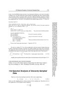
13.1 Convolution and Deconvolution Using
the FFT
We have defined the convolution of two functions for the continuous case in
equation (12.0.8), and have given the convolution theorem as equation (12.0.9). The
theorem says that the Fourier transform of the convolution of two functions is equal
to the product of their individual Fourier transforms. Now, we want to deal with
the discrete case. We will mention first the context in which convolution is a useful
procedure, and then discuss how to compute it efficiently using the FFT.
The convolutionof two functionsr(t) and s(t), denoted r ∗ s, is mathematically
equal to their convolution in the opposite order, s ∗ r. Nevertheless, in most
applications the two functions have quite different meanings and characters. One of
the functions, say s, is typically a signal or data stream, which goes on indefinitely
in time (or in whatever the appropriate independent variable may be). The other
function r is a “response function,” typically a peaked function that falls to zero in
both directions from its maximum. The effect of convolution is to smear the signal
s(t) in time according to the recipe provided by the response function r(t), as shown
in Figure 13.1.1. In particular, a spike or delta-functionof unit area ins which occurs
at some time t

0
is supposed to be smeared into the shape of the response function
itself, but translated from time 0 to time t
0
as r(t − t
0
).
In the discrete case, the signal s(t) is represented by its sampled values at equal
time intervals s
j
. The response functionis also a discrete set of numbers r
k
, with the
followinginterpretation: r
0
tellswhat multipleofthe input signalinone channel (one
particular value of j) is copied into the identical output channel (same value of j);
r
1
tells what multiple of input signal in channel j is additionally copied into output
channel j +1;r
−1
tells the multiplethat is copied into channel j − 1; and so on for
both positive and negative values of k in r
k
. Figure 13.1.2 illustrates the situation.
Example: a response function with r
0
=1and all other r
k

’s equal to zero
is just the identity filter: convolution of a signal with this response function gives
identically the signal. Another example is the response function with r
14
=1.5and
all other r
k
’s equal to zero. This produces convolved output that is the input signal
multiplied by 1.5 and delayed by 14 sample intervals.
Evidently, we have just described in words the following definition of discrete
convolution with a response function of finite duration M:
(r ∗ s)
j
≡
M/2

k=−M/2+1
s
j−k
r
k
(13.1.1)
If a discrete response function is nonzero only in some range −M/2 <k≤M/2,
where M is a sufficiently large even integer, then the response function is called a
finite impulse response (FIR), and its duration is M. (Notice that we are defining M
as the number of nonzero values of r
k
; these values span a time interval of M − 1
sampling times.) In most practical circumstances the case of finite M is the case of
interest, either because the responsereally has a finiteduration,or because we choose

to truncate it at some point and approximate it by a finite-durationresponse function.
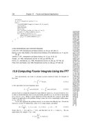
The discrete convolution theorem is this: If a signal s
j
is periodic with period
N, so that it is completely determined by the N values s
0
, ,s
N−1
, then its