Fourier and Spectral Applications part 9

13.8 Spectral Analysis of Unevenly Sampled Data
575
Sample page from NUMERICAL RECIPES IN C: THE ART OF SCIENTIFIC COMPUTING (ISBN 0-521-43108-5)
Copyright (C) 1988-1992 by Cambridge University Press.Programs Copyright (C) 1988-1992 by Numerical Recipes Software.
Permission is granted for internet users to make one paper copy for their own personal use. Further reproduction, or any copying of machine-
readable files (including this one) to any servercomputer, is strictly prohibited. To order Numerical Recipes books,diskettes, or CDROMs
visit website or call 1-800-872-7423 (North America only),or send email to (outside North America).
In fact, since the MEM estimate may have very sharpspectral features, one wants to be able to
evaluate it on a very fine mesh near to those features, but perhaps only more coarsely farther
away from them. Here is a function which, given the coefficients already computed, evaluates
(13.7.4) and returns the estimated power spectrum as a function of f∆ (the frequency times
the sampling interval). Of course, f∆ shouldlie in the Nyquist range between −1/2 and 1/2.
#include <math.h>
float evlmem(float fdt, float d[], int m, float xms)
Given
d[1..m]
,
m
,
xms
as returned by
memcof
, this function returns the power spectrum
estimate P (f ) as a function of
fdt
= f∆.
{
int i;
float sumr=1.0,sumi=0.0;
double wr=1.0,wi=0.0,wpr,wpi,wtemp,theta; Trig. recurrences in double precision.
theta=6.28318530717959*fdt;

wpr=cos(theta); Set up for recurrence relations.
wpi=sin(theta);
for (i=1;i<=m;i++) { Loop over the terms in the sum.
wr=(wtemp=wr)*wpr-wi*wpi;
wi=wi*wpr+wtemp*wpi;
sumr -= d[i]*wr; These accumulate the denominator of (13.7.4).
sumi -= d[i]*wi;
}
return xms/(sumr*sumr+sumi*sumi); Equation (13.7.4).
}
Be sure to evaluate P (f) on a fine enough grid to find any narrow features that may
be there! Such narrow features, if present, can contain virtually all of the power in the data.
You might also wish to know how the P (f) produced by the routines memcof and evlmem is
normalized with respect to the mean square value of the input data vector. The answer is

1/2
−1/2
P (f∆)d(f ∆) = 2

1/2
0
P (f ∆)d(f ∆) = mean square value of data (13.7.8)
Sample spectra producedby theroutines memcofand evlmemare shownin Figure 13.7.1.
CITED REFERENCES AND FURTHER READING:
Childers, D.G. (ed.) 1978,
Modern Spectrum Analysis
(New York: IEEE Press), Chapter II.
Kay, S.M., and Marple, S.L. 1981,
Proceedings of the IEEE
, vol. 69, pp. 1380–1419.

13.8 Spectral Analysis of Unevenly Sampled
Data
Thus far, we have been dealing exclusively with evenly sampled data,
h
n
= h(n∆) n = ...,−3,−2,−1,0,1,2,3,... (13.8.1)
where ∆ is the sampling interval, whose reciprocal is the sampling rate. Recall also (§12.1)
the significance of the Nyquist critical frequency
f
c
≡
1
2∆
(13.8.2)
576
Chapter 13. Fourier and Spectral Applications
Sample page from NUMERICAL RECIPES IN C: THE ART OF SCIENTIFIC COMPUTING (ISBN 0-521-43108-5)
Copyright (C) 1988-1992 by Cambridge University Press.Programs Copyright (C) 1988-1992 by Numerical Recipes Software.
Permission is granted for internet users to make one paper copy for their own personal use. Further reproduction, or any copying of machine-
readable files (including this one) to any servercomputer, is strictly prohibited. To order Numerical Recipes books,diskettes, or CDROMs
visit website or call 1-800-872-7423 (North America only),or send email to (outside North America).
power spectral densitty
0.1
1
10
100
1000
.1 .15 .2 .25 .3
frequency f
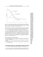
Figure 13.7.1. Sample output of maximum entropy spectral estimation. The input signal consists of

512 samples of the sum of two sinusoids of very nearly the same frequency, plus white noise with about
equal power. Shown is an expanded portion of the full Nyquist frequency interval (which would extend
from zero to 0.5). The dashed spectral estimate uses 20 poles; the dotted, 40; the solid, 150. With the
larger number of poles, the method can resolve the distinct sinusoids; but the flat noise background is
beginning to show spurious peaks. (Note logarithmic scale.)
as codified by the sampling theorem: A sampled data set like equation (13.8.1) contains
complete information about all spectral components in a signal h(t) up to the Nyquist
frequency, and scrambled or aliased information about any signal components at frequencies
larger than the Nyquist frequency. The sampling theorem thus defines both the attractiveness,
and the limitation, of any analysis of an evenly spaced data set.
There are situations, however, where evenly spaced data cannot be obtained. A common
case is where instrumental drop-outs occur, so that data is obtained only on a (not consecutive
integer) subset of equation (13.8.1), the so-called missing data problem. Another case,
common in observational sciences like astronomy, is that the observer cannot completely
control the time of the observations, but must simply accept a certain dictated set of t
i
’s.
There are some obvious ways to get from unevenlyspaced t
i
’s to evenlyspaced ones, as
in equation (13.8.1). Interpolation is one way: laydown a grid of evenly spaced times on your
data and interpolate values onto that grid; then use FFT methods. In the missing data problem,
you only have to interpolate on missing data points. If a lot of consecutive points are missing,
youmight as well justset themto zero, or perhaps“clamp” the valueat the last measuredpoint.
However, the experience of practitioners of such interpolation techniques is not reassuring.
Generally speaking, such techniques perform poorly. Long gaps in the data, for example,
often producea spurious bulgeof powerat low frequencies(wavelengths comparableto gaps).
A completely different method of spectral analysis for unevenly sampled data, one that
mitigates these difficulties and has some other very desirable properties, was developed by
Lomb

[1]
, based in part on earlier work by Barning
[2]
and Van´ıˇcek
[3]
, and additionally
elaborated by Scargle
[4]
. The Lomb method (as we will call it) evaluates data, and sines
13.8 Spectral Analysis of Unevenly Sampled Data
577
Sample page from NUMERICAL RECIPES IN C: THE ART OF SCIENTIFIC COMPUTING (ISBN 0-521-43108-5)
Copyright (C) 1988-1992 by Cambridge University Press.Programs Copyright (C) 1988-1992 by Numerical Recipes Software.
Permission is granted for internet users to make one paper copy for their own personal use. Further reproduction, or any copying of machine-
readable files (including this one) to any servercomputer, is strictly prohibited. To order Numerical Recipes books,diskettes, or CDROMs
visit website or call 1-800-872-7423 (North America only),or send email to (outside North America).
and cosines, only at times t
i
that are actually measured. Suppose that there are N data
points h
i
≡ h(t
i
),i=1,...,N. Then first find the mean and variance of the data by
the usual formulas,
h ≡
1
N
N


1
h
i
σ
2
≡
1
N − 1
N

1
(h
i
− h)
2
(13.8.3)
Now, the Lomb normalized periodogram (spectral power as a function of angular
frequency ω ≡ 2πf > 0)isdefinedby
P
N
(ω)≡
1
2σ
2








j
(h
j
−h)cosω(t
j
−τ)

2

j
cos
2
ω(t
j
− τ )
+


j
(h
j
− h)sinω(t
j
−τ)

2

j
sin

2
ω(t
j
− τ)





(13.8.4)
Here τ is defined by the relation
tan(2ωτ)=

j
sin 2ωt
j

j
cos 2ωt
j
(13.8.5)
The constant τ is a kind of offset that makes P
N
(ω) completely independentof shifting
all the t
i
’s by any constant. Lomb shows that this particular choice of offset has another,
deeper, effect: It makesequation (13.8.4) identical to the equationthat one would obtain if one
estimated the harmonic content of a data set, at a given frequency ω, by linear least-squares
fitting to the model

h(t)=Acos ωt + B sin ωt (13.8.6)
This fact gives some insight into why the method can give results superior to FFT methods: It
weights the data on a “per point” basis instead of on a “per time interval” basis, when uneven
sampling can render the latter seriously in error.
A very common occurrence is that the measured data points h
i
are the sum of a periodic
signal and independent (white) Gaussian noise. If we are trying to determine the presence
or absence of such a periodic signal, we want to be able to give a quantitative answer to
the question, “How significant is a peak in the spectrum P
N
(ω)?” In this question, the null
hypothesis is that the data values are independent Gaussian random values. A very nice
property of the Lomb normalized periodogram is that the viability of the null hypothesis can
be tested fairly rigorously, as we now discuss.
The word “normalized” refers to the factor σ
2
in the denominator of equation (13.8.4).
Scargle
[4]
shows that with this normalization, at any particular ω and in the case of the null
hypothesis, P
N
(ω) has an exponential probability distribution with unit mean. In other words,
the probability that P
N
(ω) will be between some positive z and z + dz is exp(−z)dz.It
readily follows that, if we scan some M independent frequencies, the probability that none
give values larger than z is (1 − e
−z

)
M
.So
P(>z)≡1−(1 − e
−z
)
M
(13.8.7)
is the false-alarm probability of the null hypothesis, that is, the significance level of any peak
in P
N
(ω) that we do see. A small value for the false-alarm probability indicates a highly
significant periodic signal.
To evaluate this significance, we need to know M. After all, the more frequencies we
look at, the less significant is some one modest bump in the spectrum. (Look long enough,
find anything!) A typical procedure will be to plot P
N
(ω) as a function of many closely
spaced frequencies in some large frequency range. How many of these are independent?
Before answering, let us first see how accurately we need to know M. The interesting
region is where the significance is a small (significant) number,  1. There, equation(13.8.7)
can be series expanded to give
P (>z)≈Me
−z
(13.8.8)
578
Chapter 13. Fourier and Spectral Applications
Sample page from NUMERICAL RECIPES IN C: THE ART OF SCIENTIFIC COMPUTING (ISBN 0-521-43108-5)
Copyright (C) 1988-1992 by Cambridge University Press.Programs Copyright (C) 1988-1992 by Numerical Recipes Software.
Permission is granted for internet users to make one paper copy for their own personal use. Further reproduction, or any copying of machine-

readable files (including this one) to any servercomputer, is strictly prohibited. To order Numerical Recipes books,diskettes, or CDROMs
visit website or call 1-800-872-7423 (North America only),or send email to (outside North America).
−2
−1
0
1
2
0102030
40
50 60 70 80
90
100
time
amplitude
.001
.005
.01
.05
.1
.5
0
2
4
6
8
10
12
14
power
0.1.2.3.4.5.6.7.8.9 1

frequency
significance levels
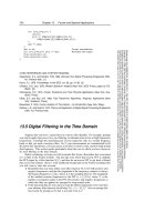
Figure 13.8.1. Example of the Lomb algorithm in action. The 100 data points (upper figure) are at
random times between 0 and 100. Their sinusoidal component is readily uncovered (lower figure) by
the algorithm, at a significance level better than 0.001. If the 100 data points had been evenly spaced at
unit interval, the Nyquist critical frequency would have been 0.5. Note that, for these unevenly spaced
points, there is no visible aliasing into the Nyquist range.
We see that the significance scales linearly with M. Practical significance levels are numbers
like 0.05, 0.01, 0.001,etc. Anerrorofeven±50% in the estimated significance is often
tolerable, since quoted significance levels are typically spaced apart by factors of 5 or 10. So
our estimate of M need not be very accurate.
Horne and Baliunas
[5]
give results from extensive Monte Carlo experiments for
determining M in various cases. In general M depends on the number of frequencies
sampled, the number of data points N, and their detailed spacing. It turns out that M is
very nearly equal to N when the data points are approximately equally spaced, and when the
sampled frequencies “fill” (oversample) the frequency range from 0 to the Nyquist frequency
f
c
(equation 13.8.2). Further, the value of M is not importantly different for random
spacing of the data points than for equal spacing. When a larger frequency range than the
Nyquist range is sampled, M increases proportionally. About the only case where M differs
significantly from the case of evenly spaced points is when the points are closely clumped,
say into groups of 3; then (as one would expect) the number of independent frequencies is
reduced by a factor of about 3.
The program period, below, calculates an effective value for M based on the above
rough-and-ready rules and assumesthat there is no important clumping. This will be adequate
for most purposes. In any particular case, if it really matters, it is not too difficult to compute
a better value of M by simple Monte Carlo: Holding fixed the number of data points and their

locations t
i
, generate synthetic data sets of Gaussian(normal) deviates, find the largest values
of P
N
(ω) for each such data set (using the accompanying program), and fit the resulting
distribution for M in equation (13.8.7).
13.8 Spectral Analysis of Unevenly Sampled Data
579
Sample page from NUMERICAL RECIPES IN C: THE ART OF SCIENTIFIC COMPUTING (ISBN 0-521-43108-5)
Copyright (C) 1988-1992 by Cambridge University Press.Programs Copyright (C) 1988-1992 by Numerical Recipes Software.
Permission is granted for internet users to make one paper copy for their own personal use. Further reproduction, or any copying of machine-
readable files (including this one) to any servercomputer, is strictly prohibited. To order Numerical Recipes books,diskettes, or CDROMs
visit website or call 1-800-872-7423 (North America only),or send email to (outside North America).
Figure 13.8.1 shows the results of applying the method as discussed so far. In the
upper figure, the data points are plotted against time. Their number is N = 100,andtheir
distribution in t is Poisson random. There is certainly no sinusoidal signal evident to the eye.
The lower figure plots P
N
(ω) against frequency f = ω/2π. The Nyquist critical frequency
that would obtain ifthe points were evenlyspaced is at f = f
c
=0.5. Since we havesearched
up to abouttwice that frequency,and oversampled the f’s to the point where successivevalues
of P
N
(ω) vary smoothly, we take M =2N. The horizontal dashed and dotted lines are
(respectively from bottom to top) significance levels 0.5, 0.1, 0.05, 0.01, 0.005, and 0.001.
One sees a highly significant peak at a frequency of 0.81. That is in fact the frequency of the
sine wave that is present in the data. (You will have to take our word for this!)

Note that two other peaks approach, but do not exceed the 50% significance level; that
is about what one might expect by chance. It is also worth commenting on the fact that the
significantpeak was found(correctly) above the Nyquistfrequencyand without any significant
aliasing down into the Nyquist interval! That would not be possible for evenly spaceddata. It
is possible here because the randomly spaced data has some points spaced much closer than
the “average” sampling rate, and these remove ambiguity from any aliasing.
Implementationofthenormalized periodogramin code isstraightforward,with,however,
a few points to be kept in mind. We are dealing with a slow algorithm. Typically, for N data
points, we may wish to examine on the order of 2N or 4N frequencies. Each combination
of frequency and data point has, in equations (13.8.4) and (13.8.5), not just a few adds or
multiplies, but four calls to trigonometric functions; the operations count can easily reach
several hundred times N
2
. It is highly desirable — in fact results in a factor 4 speedup —
to replace these trigonometric calls by recurrences. That is possible only if the sequence of
frequencies examined is a linear sequence. Since sucha sequenceis probably what most users
would want anyway, we have built this into the implementation.
At the end of this section we describe a way to evaluate equations (13.8.4) and (13.8.5)
— approximately, but to any desired degree of approximation — by a fast method
[6]
whose
operation count goes only as N log N. This faster method should be used for long data sets.
The lowest independent frequency f to be examined is the inverse of the span of the
input data, max
i
(t
i
) − min
i
(t

i
) ≡ T. This is the frequency such that the data can include one
complete cycle. In subtracting off the data’s mean, equation (13.8.4) already assumed that you
are not interested in the data’s zero-frequency piece — which is just that mean value. In an
FFT method, higher independent frequencies would be integer multiples of 1/T. Because we
are interested in thestatistical significance of any peak that may occur, however, we had better
(over-) sample more finely than at interval 1/T, so that sample points lie close to the top of
anypeak. Thus,the accompanyingprogram includes an oversamplingparameter, called ofac;
avalueofac
>
∼
4 might be typical in use. We also want to specify how high in frequency
to go, say f
hi
. One guide to choosing f
hi
is to compare it with the Nyquist frequency f
c
which would obtain if the N data points were evenly spaced over the same span T,thatis
f
c
=N/(2T ). The accompanying program includes an input parameter hifac,definedas
f
hi
/f
c
. The number of different frequencies N
P
returned by the program is then given by
N

P
=
ofac × hifac
2
N (13.8.9)
(You have to remember to dimension the output arrays to at least this size.)
The code does the trigonometric recurrences in double precision and embodies a few
tricks with trigonometric identities, to decrease roundoff errors. If you are an aficionado of
such things you can puzzle it out. A final detail is that equation (13.8.7) will fail because of
roundoff error if z is too large; but equation (13.8.8) is fine in this regime.
#include <math.h>
#include "nrutil.h"
#define TWOPID 6.2831853071795865
void period(float x[], float y[], int n, float ofac, float hifac, float px[],
float py[], int np, int *nout, int *jmax, float *prob)
Given
n
data points with abscissas
x[1..n]
(which need not be equally spaced) and ordinates
y[1..n]
, and given a desired oversampling factor
ofac
(a typical value being 4 or larger),
this routine fills array
px[1..np]
with an increasing sequence of frequencies (not angular