Fourier and Spectral Applications part 10

584
Chapter 13. Fourier and Spectral Applications
Sample page from NUMERICAL RECIPES IN C: THE ART OF SCIENTIFIC COMPUTING (ISBN 0-521-43108-5)
Copyright (C) 1988-1992 by Cambridge University Press.Programs Copyright (C) 1988-1992 by Numerical Recipes Software.
Permission is granted for internet users to make one paper copy for their own personal use. Further reproduction, or any copying of machine-
readable files (including this one) to any servercomputer, is strictly prohibited. To order Numerical Recipes books,diskettes, or CDROMs
visit website or call 1-800-872-7423 (North America only),or send email to (outside North America).
ix=(int)x;
if (x == (float)ix) yy[ix] += y;
else {
ilo=LMIN(LMAX((long)(x-0.5*m+1.0),1),n-m+1);
ihi=ilo+m-1;
nden=nfac[m];
fac=x-ilo;
for (j=ilo+1;j<=ihi;j++) fac *= (x-j);
yy[ihi] += y*fac/(nden*(x-ihi));
for (j=ihi-1;j>=ilo;j--) {
nden=(nden/(j+1-ilo))*(j-ihi);
yy[j] += y*fac/(nden*(x-j));
}
}
}
CITED REFERENCES AND FURTHER READING:
Lomb, N.R. 1976,
Astrophysics and Space Science
, vol. 39, pp. 447–462. [1]
Barning, F.J.M. 1963,
Bulletin of the Astronomical Institutes of the Netherlands
, vol. 17, pp. 22–
28. [2]
Van´ı

ˇ
cek, P. 1971,
Astrophysics and Space Science
, vol. 12, pp. 10–33. [3]
Scargle, J.D. 1982,
Astrophysical Journal
, vol. 263, pp. 835–853. [4]
Horne, J.H., and Baliunas, S.L. 1986,
Astrophysical Journal
, vol. 302, pp. 757–763. [5]
Press, W.H. and Rybicki, G.B. 1989,
Astrophysical Journal
, vol. 338, pp. 277–280. [6]
13.9 Computing Fourier Integrals Using the FFT
Not uncommonly, one wants to calculate accurate numerical values for integrals of
the form
I =

b
a
e
iωt
h(t)dt , (13.9.1)
or the equivalent real and imaginary parts
I
c
=

b
a

cos(ωt)h(t)dt I
s
=

b
a
sin(ωt)h(t)dt , (13.9.2)
and one wantsto evaluate this integralfor many different valuesof ω. In casesof interest, h(t)
is often a smooth function, but it is not necessarily periodic in [a, b], nor does it necessarily
go to zero at a or b. While it seems intuitively obvious that the force majeure of the FFT
ought to be applicable to this problem, doing so turns out to be a surprisingly subtle matter,
as we will now see.
Let us first approach the problem naively, to see where the difficulty lies. Divide the
interval [a, b] into M subintervals, where M is a large integer, and define
∆ ≡
b − a
M
,t
j
≡a+j∆,h
j
≡h(t
j
),j=0,...,M (13.9.3)
Notice that h
0
= h(a) and h
M
= h(b), and that there are M +1values h
j

. We can
approximate the integral I by a sum,
I ≈ ∆
M −1

j=0
h
j
exp(iωt
j
)(13.9.4)
13.9 Computing Fourier Integrals Using the FFT
585
Sample page from NUMERICAL RECIPES IN C: THE ART OF SCIENTIFIC COMPUTING (ISBN 0-521-43108-5)
Copyright (C) 1988-1992 by Cambridge University Press.Programs Copyright (C) 1988-1992 by Numerical Recipes Software.
Permission is granted for internet users to make one paper copy for their own personal use. Further reproduction, or any copying of machine-
readable files (including this one) to any servercomputer, is strictly prohibited. To order Numerical Recipes books,diskettes, or CDROMs
visit website or call 1-800-872-7423 (North America only),or send email to (outside North America).
which is at any rate first-order accurate. (If we centered the h
j
’s and the t
j
’s in the intervals,
we could be accurate to second order.) Now for certain values of ω and M,thesumin
equation (13.9.4) can be made into a discrete Fourier transform, or DFT, and evaluated by
the fast Fourier transform (FFT) algorithm. In particular, we can choose M to be an integer
power of 2, and define a set of special ω’s by
ω
m
∆ ≡

2πm
M
(13.9.5)
where m has the values m =0,1,...,M/2−1. Then equation (13.9.4) becomes
I(ω
m
) ≈ ∆e
iω
m
a
M −1

j=0
h
j
e
2πimj/M
=∆e
iω
m
a
[DFT(h
0
...h
M−1
)]
m
(13.9.6)
Equation (13.9.6), while simple and clear, is emphatically not recommended for use: It is
likely to give wrong answers!

The problem lies in the oscillatory nature of the integral (13.9.1). If h(t) is at allsmooth,
and if ω is large enough to imply severalcycles in the interval [a, b] — in fact, ω
m
in equation
(13.9.5) gives exactly m cycles — then the value of I is typically very small, so small that
it is easily swamped by first-order, or even (with centered values) second-order, truncation
error. Furthermore, the characteristic “small parameter” that occurs in the error term is not
∆/(b − a)=1/M, as it would be if the integrand were not oscillatory, but ω∆, which can be
as large as π for ω’s within the Nyquist interval of the DFT (cf. equation 13.9.5). The result
is that equation (13.9.6) becomes systematically inaccurate as ω increases.
It is a sobering exercise to implement equation (13.9.6) for an integral that can be done
analytically, and to see just how bad it is. We recommend that you try it.
Let us therefore turn to a more sophisticatedtreatment. Given the sampled points h
j
,we
can approximate the function h(t) everywhere in the interval [a, b] by interpolation on nearby
h
j
’s. The simplest case is linear interpolation, using the two nearest h
j
’s, one to the left and
one to the right. A higher-order interpolation, e.g., would be cubic interpolation, using two
points to the left and two to the right — except in the first and last subintervals, where we
must interpolate with three h
j
’s on one side, one on the other.
The formulas for such interpolation schemes are (piecewise) polynomial in the inde-
pendent variable t, but with coefficients that are of course linear in the function values
h
j

. Although one does not usually think of it in this way, interpolation can be viewed as
approximatinga function by a sum ofkernelfunctions (whichdependonly on the interpolation
scheme) times sample values (which depend only on the function). Let us write
h(t) ≈
M

j=0
h
j
ψ

t − t
j
∆

+

j=endpoints
h
j
ϕ
j

t − t
j
∆

(13.9.7)
Here ψ(s) is the kernel function of an interior point: It is zero for s sufficiently negative
or sufficiently positive, and becomes nonzero only when s is in the range where the

h
j
multiplying it is actually used in the interpolation. We always have ψ(0) = 1 and
ψ(m)=0,m=±1,±2,..., since interpolation right on a sample point should give the
sampled function value. For linear interpolation ψ(s) is piecewise linear, rises from 0 to 1
for s in (−1, 0), and falls back to 0 for s in (0, 1). For higher-order interpolation, ψ(s) is
made up piecewise of segments of Lagrange interpolation polynomials. It has discontinuous
derivatives at integer values of s, where the pieces join, because the set of points used in
the interpolation changes discretely.
As already remarked, the subintervals closest to a and b require different (noncentered)
interpolation formulas. This is reflected in equation (13.9.7) by the second sum, with the
specialendpoint kernels ϕ
j
(s). Actually, for reasons that will become clearer below, we have
included all the points in the first sum (with kernel ψ), so the ϕ
j
’s are actually differences
between true endpoint kernels and the interior kernel ψ. It is a tedious, but straightforward,
exercise to write down all the ϕ
j
(s)’s for any particular order of interpolation, each one
consisting of differences of Lagrange interpolating polynomials spliced together piecewise.
Now apply the integral operator

b
a
dt exp(iωt) to both sides of equation (13.9.7),
interchange the sums and integral, and make the changes of variable s =(t−t
j
)/∆in the

586
Chapter 13. Fourier and Spectral Applications
Sample page from NUMERICAL RECIPES IN C: THE ART OF SCIENTIFIC COMPUTING (ISBN 0-521-43108-5)
Copyright (C) 1988-1992 by Cambridge University Press.Programs Copyright (C) 1988-1992 by Numerical Recipes Software.
Permission is granted for internet users to make one paper copy for their own personal use. Further reproduction, or any copying of machine-
readable files (including this one) to any servercomputer, is strictly prohibited. To order Numerical Recipes books,diskettes, or CDROMs
visit website or call 1-800-872-7423 (North America only),or send email to (outside North America).
first sum, s =(t−a)/∆in the second sum. The result is
I ≈ ∆e
iωa

W (θ)
M

j=0
h
j
e
ijθ
+

j=endpoints
h
j
α
j
(θ)

(13.9.8)
Here θ ≡ ω∆, and the functions W(θ) and α

j
(θ) are defined by
W(θ) ≡

∞
−∞
ds e
iθs
ψ(s)(13.9.9)
α
j
(θ) ≡

∞
−∞
ds e
iθs
ϕ
j
(s − j)(13.9.10)
The key point is that equations (13.9.9) and (13.9.10) can be evaluated, analytically,
once and for all, for any given interpolation scheme. Then equation (13.9.8) is an algorithm
for applying “endpoint corrections” to a sum which (as we will see) can be done using the
FFT, giving a result with high-order accuracy.
We will consider only interpolations that are left-right symmetric. Then symmetry
implies
ϕ
M −j
(s)=ϕ
j

(−s) α
M−j
(θ)=e
iθM
α
*
j
(θ)=e
iω(b−a)
α
*
j
(θ)(13.9.11)
where * denotes complex conjugation. Also, ψ(s)=ψ(−s)implies that W (θ) is real.
Turn now to the first sum in equation (13.9.8), which we want to do by FFT methods.
To do so, choose some N that is an integer power of 2 with N ≥ M +1. (Note that
M need not be a power of two, so M = N − 1 is allowed.) If N>M+1,define
h
j
≡0,M+1<j≤N−1, i.e., “zero pad” the array of h
j
’s so that j takes on the range
0 ≤ j ≤ N − 1. Then the sum can be done as a DFT for the special values ω = ω
n
given by
ω
n
∆ ≡
2πn
N

≡ θn=0,1,...,
N
2
−1(13.9.12)
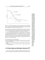
For fixed M,thelargerNis chosen, the finer the sampling in frequency space. The
value M, on the other hand, determines the highest frequency sampled, since ∆ decreases
with increasing M (equation 13.9.3), and the largest value of ω∆ is always just under π
(equation 13.9.12). In general it is advantageous to oversample by at least a factor of 4, i.e.,
N>4M(see below). We can now rewrite equation (13.9.8) in its final form as
I(ω
n
)=∆e
iω
n
a

W (θ)[DFT(h
0
...h
N−1
)]
n
+ α
0
(θ)h
0
+ α
1
(θ)h
1

+ α
2
(θ)h
2
+ α
3
(θ)h
3
+ ...
+e
iω(b−a)

α
*
0
(θ)h
M
+ α
*
1
(θ)h
M −1
+ α
*
2
(θ)h
M −2
+ α
*
3

(θ)h
M −3
+ ...


(13.9.13)
For cubic (or lower) polynomial interpolation, at most the terms explicitly shown above
are nonzero; the ellipses (...) can therefore be ignored, and we need explicit forms only for
the functions W, α
0
,α
1
,α
2
,α
3
, calculated with equations (13.9.9) and (13.9.10). We have
worked these out for you, in the trapezoidal (second-order) and cubic (fourth-order) cases.
Here are the results, along with the first few terms of their power series expansionsfor small θ:
Trapezoidal order:
W (θ)=
2(1 − cos θ)
θ
2
≈ 1 −
1
12
θ
2
+

1
360
θ
4
−
1
20160
θ
6
α
0
(θ)=−
(1 − cos θ)
θ
2
+ i
(θ − sin θ)
θ
2
≈−
1
2
+
1
24
θ
2
−
1
720

θ
4
+
1
40320
θ
6
+ iθ

1
6
−
1
120
θ
2
+
1
5040
θ
4
−
1
362880
θ
6

α
1
= α

2
= α
3
=0
13.9 Computing Fourier Integrals Using the FFT
587
Sample page from NUMERICAL RECIPES IN C: THE ART OF SCIENTIFIC COMPUTING (ISBN 0-521-43108-5)
Copyright (C) 1988-1992 by Cambridge University Press.Programs Copyright (C) 1988-1992 by Numerical Recipes Software.
Permission is granted for internet users to make one paper copy for their own personal use. Further reproduction, or any copying of machine-
readable files (including this one) to any servercomputer, is strictly prohibited. To order Numerical Recipes books,diskettes, or CDROMs
visit website or call 1-800-872-7423 (North America only),or send email to (outside North America).
Cubic order:
W (θ)=

6+θ
2
3θ
4

(3 − 4cosθ+cos2θ)≈1−
11
720
θ
4
+
23
15120
θ
6
α

0
(θ)=
(−42 + 5θ
2
)+(6+θ
2
)(8 cos θ − cos 2θ)
6θ
4
+ i
(−12θ +6θ
3
)+(6+θ
2
)sin2θ
6θ
4
≈−
2
3
+
1
45
θ
2
+
103
15120
θ
4

−
169
226800
θ
6
+ iθ

2
45
+
2
105
θ
2
−
8
2835
θ
4
+
86
467775
θ
6

α
1
(θ)=
14(3 − θ
2

) − 7(6 + θ
2
)cosθ
6θ
4
+i
30θ − 5(6 + θ
2
)sinθ
6θ
4
≈
7
24
−
7
180
θ
2
+
5
3456
θ
4
−
7
259200
θ
6
+ iθ


7
72
−
1
168
θ
2
+
11
72576
θ
4
−
13
5987520
θ
6

α
2
(θ)=
−4(3 − θ
2
)+2(6+θ
2
)cosθ
3θ
4
+i

−12θ +2(6+θ
2
)sinθ
3θ
4
≈−
1
6
+
1
45
θ
2
−
5
6048
θ
4
+
1
64800
θ
6
+ iθ

−
7
90
+
1

210
θ
2
−
11
90720
θ
4
+
13
7484400
θ
6

α
3
(θ)=
2(3 − θ
2
) − (6 + θ
2
)cosθ
6θ
4
+i
6θ −(6 + θ
2
)sinθ
6θ
4

≈
1
24
−
1
180
θ
2
+
5
24192
θ
4
−
1
259200
θ
6
+ iθ

7
360
−
1
840
θ
2
+
11
362880

θ
4
−
13
29937600
θ
6

The program dftcor, below, implements the endpoint corrections for the cubic case.
Given inputvaluesof ω,∆,a,b,and an array with the eight values h
0
,...,h
3
,h
M−3
,...,h
M
,
it returns therealand imaginary parts of the endpointcorrections in equation (13.9.13), and the
factor W(θ). The code is turgid, but only because the formulas above are complicated. The
formulas have cancellationsto high powers of θ. It istherefore necessarytocompute the right-
hand sides in double precision, even whenthe corrections are desired only to single precision.
It is also necessary to use the series expansion for small values of θ. The optimal cross-over
value of θ depends on your machine’s wordlength, but you can always find it experimentally
as the largest value where the two methods give identical results to machine precision.
#include <math.h>
void dftcor(float w, float delta, float a, float b, float endpts[],
float *corre, float *corim, float *corfac)
For an integral approximated by a discrete Fourier transform, this routine computes the cor-
rection factor that multiplies the DFT and the endpoint correction to be added. Input is the

angular frequency
w
,stepsize
delta
, lower and upper limits of the integral
a
and
b
, while the
array
endpts
contains the first 4 and last 4 function values. The correction factor W (θ) is
returned as
corfac
, while the real and imaginary parts of the endpoint correction are returned
as
corre
and
corim
.
{
void nrerror(char error_text[]);
float a0i,a0r,a1i,a1r,a2i,a2r,a3i,a3r,arg,c,cl,cr,s,sl,sr,t;
float t2,t4,t6;
double cth,ctth,spth2,sth,sth4i,stth,th,th2,th4,tmth2,tth4i;
th=w*delta;
if (a >= b || th < 0.0e0 || th > 3.01416e0) nrerror("bad arguments to dftcor");
if (fabs(th) < 5.0e-2) { Use series.
t=th;
t2=t*t;

t4=t2*t2;
t6=t4*t2;
588
Chapter 13. Fourier and Spectral Applications
Sample page from NUMERICAL RECIPES IN C: THE ART OF SCIENTIFIC COMPUTING (ISBN 0-521-43108-5)
Copyright (C) 1988-1992 by Cambridge University Press.Programs Copyright (C) 1988-1992 by Numerical Recipes Software.
Permission is granted for internet users to make one paper copy for their own personal use. Further reproduction, or any copying of machine-
readable files (including this one) to any servercomputer, is strictly prohibited. To order Numerical Recipes books,diskettes, or CDROMs
visit website or call 1-800-872-7423 (North America only),or send email to (outside North America).
*corfac=1.0-(11.0/720.0)*t4+(23.0/15120.0)*t6;
a0r=(-2.0/3.0)+t2/45.0+(103.0/15120.0)*t4-(169.0/226800.0)*t6;
a1r=(7.0/24.0)-(7.0/180.0)*t2+(5.0/3456.0)*t4-(7.0/259200.0)*t6;
a2r=(-1.0/6.0)+t2/45.0-(5.0/6048.0)*t4+t6/64800.0;
a3r=(1.0/24.0)-t2/180.0+(5.0/24192.0)*t4-t6/259200.0;
a0i=t*(2.0/45.0+(2.0/105.0)*t2-(8.0/2835.0)*t4+(86.0/467775.0)*t6);
a1i=t*(7.0/72.0-t2/168.0+(11.0/72576.0)*t4-(13.0/5987520.0)*t6);
a2i=t*(-7.0/90.0+t2/210.0-(11.0/90720.0)*t4+(13.0/7484400.0)*t6);
a3i=t*(7.0/360.0-t2/840.0+(11.0/362880.0)*t4-(13.0/29937600.0)*t6);
} else { Use trigonometric formulas in double precision.
cth=cos(th);
sth=sin(th);
ctth=cth*cth-sth*sth;
stth=2.0e0*sth*cth;
th2=th*th;
th4=th2*th2;
tmth2=3.0e0-th2;
spth2=6.0e0+th2;
sth4i=1.0/(6.0e0*th4);
tth4i=2.0e0*sth4i;
*corfac=tth4i*spth2*(3.0e0-4.0e0*cth+ctth);

a0r=sth4i*(-42.0e0+5.0e0*th2+spth2*(8.0e0*cth-ctth));
a0i=sth4i*(th*(-12.0e0+6.0e0*th2)+spth2*stth);
a1r=sth4i*(14.0e0*tmth2-7.0e0*spth2*cth);
a1i=sth4i*(30.0e0*th-5.0e0*spth2*sth);
a2r=tth4i*(-4.0e0*tmth2+2.0e0*spth2*cth);
a2i=tth4i*(-12.0e0*th+2.0e0*spth2*sth);
a3r=sth4i*(2.0e0*tmth2-spth2*cth);
a3i=sth4i*(6.0e0*th-spth2*sth);
}
cl=a0r*endpts[1]+a1r*endpts[2]+a2r*endpts[3]+a3r*endpts[4];
sl=a0i*endpts[1]+a1i*endpts[2]+a2i*endpts[3]+a3i*endpts[4];
cr=a0r*endpts[8]+a1r*endpts[7]+a2r*endpts[6]+a3r*endpts[5];
sr = -a0i*endpts[8]-a1i*endpts[7]-a2i*endpts[6]-a3i*endpts[5];
arg=w*(b-a);
c=cos(arg);
s=sin(arg);
*corre=cl+c*cr-s*sr;
*corim=sl+s*cr+c*sr;
}
Since the use of dftcor can be confusing, we also give an illustrative program dftint
which uses dftcor to compute equation (13.9.1) for general a, b, ω,andh(t). Several points
within this program bear mentioning: The parameters M and NDFT correspond to M and N
in the above discussion. On successive calls, we recompute the Fourier transform only if
a or b or h(t) has changed.
Since dftint is designed to work for any value of ω satisfying ω∆ <π, not just the
special values returned by the DFT (equation 13.9.12), we do polynomial interpolation of
degree MPOL on the DFT spectrum. You should be warned that a large factor of oversampling
(N  M) is required for this interpolation to be accurate. After interpolation, we add the
endpoint corrections from dftcor, which can be evaluated for any ω.
While dftcor is good at what it does, dftint is illustrative only. It is not a general

purpose program, because it does not adapt its parameters M, NDFT, MPOL, or its interpolation
scheme, to any particular function h(t). You will have to experiment with your own
application.
#include <math.h>
#include "nrutil.h"
#define M 64
#define NDFT 1024
#define MPOL 6
#define TWOPI (2.0*3.14159265)