Tài liệu Sorting and Searching Algorithms: A Cookbook doc
Bạn đang xem bản rút gọn của tài liệu. Xem và tải ngay bản đầy đủ của tài liệu tại đây (158.57 KB, 36 trang )
Sorting and Searching Algorithms:
A Cookbook
Thomas Niemann
- 2 -
Preface
This is a collection of algorithms for sorting and searching. Descriptions are brief and intuitive,
with just enough theory thrown in to make you nervous. I assume you know C, and that you are
familiar with concepts such as arrays and pointers.
The first section introduces basic data structures and notation. The next section presents
several sorting algorithms. This is followed by techniques for implementing dictionaries,
structures that allow efficient search, insert, and delete operations. The last section illustrates
algorithms that sort data and implement dictionaries for very large files. Source code for each
algorithm, in ANSI C, is available at the site listed below.
Permission to reproduce this document, in whole or in part, is given provided the original
web site listed below is referenced, and no additional restrictions apply. Source code, when part
of a software project, may be used freely without reference to the author.
THOMAS NIEMANN
Portland, Oregon
email:
home: />By the same author:
A Guide to Lex and Yacc, at />- 3 -
CONTENTS
1. INTRODUCTION 4
2. SORTING 8
2.1 Insertion Sort 8
2.2 Shell Sort 10
2.3 Quicksort 11
2.4 Comparison 14
3. DICTIONARIES 15
3.1 Hash Tables 15
3.2 Binary Search Trees 19
3.3 Red-Black Trees 21
3.4 Skip Lists 25
3.5 Comparison 26
4. VERY LARGE FILES 29
4.1 External Sorting 29
4.2 B-Trees 32
5. BIBLIOGRAPHY 36
- 4 -
1. Introduction
Arrays and linked lists are two basic data structures used to store information. We may wish to
search, insert or delete records in a database based on a key value. This section examines the
performance of these operations on arrays and linked lists.
Arrays
Figure 1-1 shows an array, seven elements long, containing numeric values. To search the array
sequentially, we may use the algorithm in Figure 1-2. The maximum number of comparisons is
7, and occurs when the key we are searching for is in A[6].
4
7
16
20
37
38
43
0
1
2
3
4
5
6
Ub
M
Lb
Figure 1-1: An Array
Figure 1-2: Sequential Search
int function SequentialSearch (Array A , int Lb , int Ub , int Key );
begin
for i = Lb to Ub do
if A [ i ] = Key then
return i ;
return –1;
end;
- 5 -
Figure 1-3: Binary Search
If the data is sorted, a binary search may be done (Figure 1-3). Variables Lb and Ub keep
track of the lower bound and upper bound of the array, respectively. We begin by examining the
middle element of the array. If the key we are searching for is less than the middle element, then
it must reside in the top half of the array. Thus, we set Ub to (M – 1). This restricts our next
iteration through the loop to the top half of the array. In this way, each iteration halves the size
of the array to be searched. For example, the first iteration will leave 3 items to test. After the
second iteration, there will be one item left to test. Therefore it takes only three iterations to find
any number.
This is a powerful method. Given an array of 1023 elements, we can narrow the search to
511 elements in one comparison. After another comparison, and we’re looking at only 255
elements. In fact, we can search the entire array in only 10 comparisons.
In addition to searching, we may wish to insert or delete entries. Unfortunately, an array is
not a good arrangement for these operations. For example, to insert the number 18 in Figure 1-1,
we would need to shift A[3]…A[6] down by one slot. Then we could copy number 18 into A[3].
A similar problem arises when deleting numbers. To improve the efficiency of insert and delete
operations, linked lists may be used.
int function BinarySearch (Array A , int Lb , int Ub , int Key );
begin
do forever
M = ( Lb + Ub )/2;
if ( Key < A[M]) then
Ub = M – 1;
else if (Key > A[M]) then
Lb = M + 1;
else
return M ;
if (Lb > Ub) then
return –1;
end;
- 6 -
Linked Lists
4 7 16 20 37 38
#
43
18
X
P
Figure 1-4: A Linked List
In Figure 1-4 we have the same values stored in a linked list. Assuming pointers X and P, as
shown in the figure, value 18 may be inserted as follows:
X->Next = P->Next;
P->Next = X;
Insertion and deletion operations are very efficient using linked lists. You may be wondering
how pointer P was set in the first place. Well, we had to do a sequential search to find the
insertion point X. Although we improved our performance for insertion/deletion, it was done at
the expense of search time.
Timing Estimates
Several methods may be used to compare the performance of algorithms. One way is simply to
run several tests for each algorithm and compare the timings. Another way is to estimate the
time required. For example, we may state that search time is O(n) (big-oh of n). This means that
search time, for large n, is proportional to the number of items n in the list. Consequently, we
would expect search time to triple if our list increased in size by a factor of three. The big-O
notation does not describe the exact time that an algorithm takes, but only indicates an upper
bound on execution time within a constant factor. If an algorithm takes O(n
2
) time, then
execution time grows no worse than the square of the size of the list.
- 7 -
n
lg
nn
lg
nn
1.25
n
2
10 0 1 1
16 4 64 32 256
256 8 2,048 1,024 65,536
4,096 12 49,152 32,768 16,777,216
65,536 16 1,048,565 1,048,476 4,294,967,296
1,048,476 20 20,969,520 33,554,432 1,099,301,922,576
16,775,616 24 402,614,784 1,073,613,825 281,421,292,179,456
Table 1-1: Growth Rates
Table 1-1 illustrates growth rates for various functions. A growth rate of O(lg n) occurs for
algorithms similar to the binary search. The lg (logarithm, base 2) function increases by one
when n is doubled. Recall that we can search twice as many items with one more comparison in
the binary search. Thus the binary search is a O(lg n) algorithm.
If the values in Table 1-1 represented microseconds, then a O(lg n) algorithm may take 20
microseconds to process 1,048,476 items, a O(n
1.25
) algorithm might take 33 seconds, and a
O(n
2
) algorithm might take up to 12 days! In the following chapters a timing estimate for each
algorithm, using big-O notation, will be included. For a more formal derivation of these
formulas you may wish to consult the references.
Summary
As we have seen, sorted arrays may be searched efficiently using a binary search. However, we
must have a sorted array to start with. In the next section various ways to sort arrays will be
examined. It turns out that this is computationally expensive, and considerable research has been
done to make sorting algorithms as efficient as possible.
Linked lists improved the efficiency of insert and delete operations, but searches were
sequential and time-consuming. Algorithms exist that do all three operations efficiently, and
they will be the discussed in the section on dictionaries.
- 8 -
2. Sorting
Several algorithms are presented, including insertion sort, shell sort, and quicksort. Sorting by
insertion is the simplest method, and doesn’t require any additional storage. Shell sort is a
simple modification that improves performance significantly. Probably the most efficient and
popular method is quicksort, and is the method of choice for large arrays.
2.1 Insertion Sort
One of the simplest methods to sort an array is an insertion sort. An example of an insertion sort
occurs in everyday life while playing cards. To sort the cards in your hand you extract a card,
shift the remaining cards, and then insert the extracted card in the correct place. This process is
repeated until all the cards are in the correct sequence. Both average and worst-case time is
O(n
2
). For further reading, consult Knuth [1998].
- 9 -
Theory
Starting near the top of the array in Figure 2-1(a), we extract the 3. Then the above elements are
shifted down until we find the correct place to insert the 3. This process repeats in Figure 2-1(b)
with the next number. Finally, in Figure 2-1(c), we complete the sort by inserting 2 in the
correct place.
4
1
2
4
3
1
2
4
1
2
3
4
1
2
3
4
2
3
4
1
2
3
4
2
1
3
4
2
1
3
4
1
3
4
2
1
3
4
1
2
3
4
D
E
F
Figure 2-1: Insertion Sort
Assuming there are n elements in the array, we must index through n – 1 entries. For each
entry, we may need to examine and shift up to n – 1 other entries, resulting in a O(n
2
) algorithm.
The insertion sort is an in-place sort. That is, we sort the array in-place. No extra memory is
required. The insertion sort is also a stable sort. Stable sorts retain the original ordering of keys
when identical keys are present in the input data.
Implementation
Source for the insertion sort algorithm may be found in file ins.c. Typedef T and comparison
operator compGT should be altered to reflect the data stored in the table.
- 10 -
2.2 Shell Sort
Shell sort, developed by Donald L. Shell, is a non-stable in-place sort. Shell sort improves on
the efficiency of insertion sort by quickly shifting values to their destination. Average sort time
is O(n
1.25
), while worst-case time is O(n
1.5
). For further reading, consult Knuth [1998].
Theory
In Figure 2-2(a) we have an example of sorting by insertion. First we extract 1, shift 3 and 5
down one slot, and then insert the 1, for a count of 2 shifts. In the next frame, two shifts are
required before we can insert the 2. The process continues until the last frame, where a total of 2
+ 2 + 1 = 5 shifts have been made.
In Figure 2-2(b) an example of shell sort is illustrated. We begin by doing an insertion sort
using a spacing of two. In the first frame we examine numbers 3-1. Extracting 1, we shift 3
down one slot for a shift count of 1. Next we examine numbers 5-2. We extract 2, shift 5 down,
and then insert 2. After sorting with a spacing of two, a final pass is made with a spacing of one.
This is simply the traditional insertion sort. The total shift count using shell sort is 1+1+1 = 3.
By using an initial spacing larger than one, we were able to quickly shift values to their proper
destination.
1
3
5
2
3
5
1
2
1
2
3
5
1
2
3
4
1
5
3
2
3
5
1
2
1
2
3
5
1
2
3
4
2s 2s 1s
1s 1s 1s
D
E
4 4 4 5
5444
Figure 2-2: Shell Sort
Various spacings may be used to implement shell sort. Typically the array is sorted with a
large spacing, the spacing reduced, and the array sorted again. On the final sort, spacing is one.
Although the shell sort is easy to comprehend, formal analysis is difficult. In particular, optimal
spacing values elude theoreticians. Knuth has experimented with several values and recommends
that spacing h for an array of size N be based on the following formula:
Nhhhhh
ttss
≥+==
++ 211
when with stop and ,13 ,1Let
- 11 -
Thus, values of h are computed as follows:
1211)403(
401)133(
131)43(
41)13(
1
5
4
3
2
1
=+×=
=+×=
=+×=
=+×=
=
h
h
h
h
h
To sort 100 items we first find h
s
such that h
s
≥ 100. For 100 items, h
5
is selected. Our final
value (h
t
) is two steps lower, or h
3
. Therefore our sequence of h values will be 13-4-1. Once the
initial h value has been determined, subsequent values may be calculated using the formula
3/
1 ss
hh =
−
Implementation
Source for the shell sort algorithm may be found in file shl.c. Typedef T and comparison
operator compGT should be altered to reflect the data stored in the array. The central portion of
the algorithm is an insertion sort with a spacing of h.
2.3 Quicksort
Although the shell sort algorithm is significantly better than insertion sort, there is still room for
improvement. One of the most popular sorting algorithms is quicksort. Quicksort executes in
O(n lg n) on average, and O(n
2
) in the worst-case. However, with proper precautions, worst-case
behavior is very unlikely. Quicksort is a non-stable sort. It is not an in-place sort as stack space
is required. For further reading, consult Cormen [1990].
Theory
The quicksort algorithm works by partitioning the array to be sorted, then recursively sorting
each partition. In Partition (Figure 2-3), one of the array elements is selected as a pivot value.
Values smaller than the pivot value are placed to the left of the pivot, while larger values are
placed to the right.
- 12 -
Figure 2-3: Quicksort Algorithm
In Figure 2-4(a), the pivot selected is 3. Indices are run starting at both ends of the array.
One index starts on the left and selects an element that is larger than the pivot, while another
index starts on the right and selects an element that is smaller than the pivot. In this case,
numbers 4 and 1 are selected. These elements are then exchanged, as is shown in Figure 2-4(b).
This process repeats until all elements to the left of the pivot are ≤ the pivot, and all items to the
right of the pivot are ≥ the pivot. QuickSort recursively sorts the two sub-arrays, resulting in the
array shown in Figure 2-4(c).
4 2 3 5 1
1 2 3 5 4
1 2 3 4 5
D
E
F
Lb Ub
SLYRW
Lb M Lb
Figure 2-4: Quicksort Example
As the process proceeds, it may be necessary to move the pivot so that correct ordering is
maintained. In this manner, QuickSort succeeds in sorting the array. If we’re lucky the pivot
selected will be the median of all values, equally dividing the array. For a moment, let’s assume
int function Partition (Array A, int Lb, int Ub);
begin
select a pivot from A[Lb]…A[Ub];
reorder A[Lb]…A[Ub] such that:
all values to the left of the pivot are
≤
pivot
all values to the right of the pivot are
≥
pivot
return pivot position;
end;
procedure QuickSort (Array A, int Lb, int Ub);
begin
if Lb < Ub then
M = Partition (A, Lb, Ub);
QuickSort (A, Lb, M – 1);
QuickSort (A, M + 1, Ub);
end;
- 13 -
that this is the case. Since the array is split in half at each step, and Partition must eventually
examine all n elements, the run time is O(n lg n).
To find a pivot value, Partition could simply select the first element (A[Lb]). All other
values would be compared to the pivot value, and placed either to the left or right of the pivot as
appropriate. However, there is one case that fails miserably. Suppose the array was originally in
order. Partition would always select the lowest value as a pivot and split the array with one
element in the left partition, and Ub – Lb elements in the other. Each recursive call to quicksort
would only diminish the size of the array to be sorted by one. Therefore n recursive calls would
be required to do the sort, resulting in a O(n
2
) run time. One solution to this problem is to
randomly select an item as a pivot. This would make it extremely unlikely that worst-case
behavior would occur.
Implementation
The source for the quicksort algorithm may be found in file qui.c. Typedef T and comparison
operator compGT should be altered to reflect the data stored in the array. Several enhancements
have been made to the basic quicksort algorithm:
• The center element is selected as a pivot in partition. If the list is partially ordered,
this will be a good choice. Worst-case behavior occurs when the center element happens
to be the largest or smallest element each time partition is invoked.
• For short arrays, insertSort is called. Due to recursion and other overhead, quicksort
is not an efficient algorithm to use on small arrays. Consequently, any array with fewer
than 12 elements is sorted using an insertion sort. The optimal cutoff value is not critical
and varies based on the quality of generated code.
• Tail recursion occurs when the last statement in a function is a call to the function itself.
Tail recursion may be replaced by iteration, resulting in a better utilization of stack space.
This has been done with the second call to QuickSort in Figure 2-3.
• After an array is partitioned, the smallest partition is sorted first. This results in a better
utilization of stack space, as short partitions are quickly sorted and dispensed with.
Included in file qsort.c is the source for qsort, an ANSI-C standard library function usually
implemented with quicksort. Recursive calls were replaced by explicit stack operations. Table
2-1 shows timing statistics and stack utilization before and after the enhancements were applied.
count before after before after
16 103 51 540 28
256 1,630 911 912 112
4,096 34,183 20,016 1,908 168
65,536 658,003 470,737 2,436 252
time (
µ
s) stacksize
Table 2-1: Effect of Enhancements on Speed and Stack Utilization
- 14 -
2.4 Comparison
In this section we will compare the sorting algorithms covered: insertion sort, shell sort, and
quicksort. There are several factors that influence the choice of a sorting algorithm:
• Stable sort. Recall that a stable sort will leave identical keys in the same relative position
in the sorted output. Insertion sort is the only algorithm covered that is stable.
• Space. An in-place sort does not require any extra space to accomplish its task. Both
insertion sort and shell sort are in-place sorts. Quicksort requires stack space for
recursion, and therefore is not an in-place sort. Tinkering with the algorithm
considerably reduced the amount of time required.
• Time. The time required to sort a dataset can easily become astronomical (Table 1-1).
Table 2-2 shows the relative timings for each method. The time required to sort a
randomly ordered dataset is shown in Table 2-3.
• Simplicity. The number of statements required for each algorithm may be found in Table
2-2. Simpler algorithms result in fewer programming errors.
method statements average time worst-case time
insertion sort 9
O
(
n
2
)
O
(
n
2
)
shell sort 17
O
(
n
1.25
)
O
(
n
1.5
)
quicksort 21
O
(
n
lg
n
)
O
(
n
2
)
Table 2-2: Comparison of Methods
count insertion shell quicksort
16
39
µ
s45
µ
s 51
µ
s
256
4,969
µ
s 1,230
µ
s 911
µ
s
4,096 1.315 sec .033 sec .020 sec
65,536 416.437 sec 1.254 sec .461 sec
Table 2-3: Sort Timings
- 15 -
3. Dictionaries
Dictionaries are data structures that support search, insert, and delete operations. One of the
most effective representations is a hash table. Typically, a simple function is applied to the key
to determine its place in the dictionary. Also included are binary trees and red-black trees. Both
tree methods use a technique similar to the binary search algorithm to minimize the number of
comparisons during search and update operations on the dictionary. Finally, skip lists illustrate a
simple approach that utilizes random numbers to construct a dictionary.
3.1 Hash Tables
Hash tables are a simple and effective method to implement dictionaries. Average time to search
for an element is O(1), while worst-case time is O(n). Cormen [1990] and Knuth [1998] both
contain excellent discussions on hashing.
Theory
A hash table is simply an array that is addressed via a hash function. For example, in Figure 3-1,
HashTable is an array with 8 elements. Each element is a pointer to a linked list of numeric
data. The hash function for this example simply divides the data key by 8, and uses the
remainder as an index into the table. This yields a number from 0 to 7. Since the range of
indices for HashTable is 0 to 7, we are guaranteed that the index is valid.
#
#
#
#
#
#
16
11
22
#
6
27
#
19
HashTable
0
1
2
3
4
5
6
7
Figure 3-1: A Hash Table
To insert a new item in the table, we hash the key to determine which list the item goes on,
and then insert the item at the beginning of the list. For example, to insert 11, we divide 11 by 8
giving a remainder of 3. Thus, 11 goes on the list starting at HashTable[3]. To find a
- 16 -
number, we hash the number and chain down the correct list to see if it is in the table. To delete
a number, we find the number and remove the node from the linked list.
Entries in the hash table are dynamically allocated and entered on a linked list associated
with each hash table entry. This technique is known as chaining. An alternative method, where
all entries are stored in the hash table itself, is known as direct or open addressing and may be
found in the references.
If the hash function is uniform, or equally distributes the data keys among the hash table
indices, then hashing effectively subdivides the list to be searched. Worst-case behavior occurs
when all keys hash to the same index. Then we simply have a single linked list that must be
sequentially searched. Consequently, it is important to choose a good hash function. Several
methods may be used to hash key values. To illustrate the techniques, I will assume unsigned
char is 8-bits, unsigned short int is 16-bits, and unsigned long int is 32-bits.
• Division method (tablesize = prime). This technique was used in the preceding example.
A HashValue, from 0 to (HashTableSize - 1), is computed by dividing the key
value by the size of the hash table and taking the remainder. For example:
typedef int HashIndexType;
HashIndexType Hash(int Key) {
return Key % HashTableSize;
}
Selecting an appropriate HashTableSize is important to the success of this method.
For example, a HashTableSize of two would yield even hash values for even Keys,
and odd hash values for odd Keys. This is an undesirable property, as all keys would
hash to the same value if they happened to be even. If HashTableSize is a power of
two, then the hash function simply selects a subset of the Key bits as the table index. To
obtain a more random scattering, HashTableSize should be a prime number not too
close to a power of two.
• Multiplication method (tablesize = 2
n
). The multiplication method may be used for a
HashTableSize that is a power of 2. The Key is multiplied by a constant, and then the
necessary bits are extracted to index into the table. Knuth recommends using the
fractional part of the product of the key and the golden ratio, or
(
)
2/15 − . For
example, assuming a word size of 8 bits, the golden ratio is multiplied by 2
8
to obtain
158. The product of the 8-bit key and 158 results in a 16-bit integer. For a table size of
2
5
the 5 most significant bits of the least significant word are extracted for the hash value.
The following definitions may be used for the multiplication method:
- 17 -
/* 8-bit index */
typedef unsigned char HashIndexType;
static const HashIndexType K = 158;
/* 16-bit index */
typedef unsigned short int HashIndexType;
static const HashIndexType K = 40503;
/* 32-bit index */
typedef unsigned long int HashIndexType;
static const HashIndexType K = 2654435769;
/* w=bitwidth(HashIndexType), size of table=2**m */
static const int S = w - m;
HashIndexType HashValue = (HashIndexType)(K * Key) >> S;
For example, if HashTableSize is 1024 (2
10
), then a 16-bit index is sufficient and S
would be assigned a value of 16 – 10 = 6. Thus, we have:
typedef unsigned short int HashIndexType;
HashIndexType Hash(int Key) {
static const HashIndexType K = 40503;
static const int S = 6;
return (HashIndexType)(K * Key) >> S;
}
• Variable string addition method (tablesize = 256). To hash a variable-length string, each
character is added, modulo 256, to a total. A HashValue, range 0-255, is computed.
typedef unsigned char HashIndexType;
HashIndexType Hash(char *str) {
HashIndexType h = 0;
while (*str) h += *str++;
return h;
}
• Variable string exclusive-or method (tablesize = 256). This method is similar to the
addition method, but successfully distinguishes similar words and anagrams. To obtain a
hash value in the range 0-255, all bytes in the string are exclusive-or'd together.
However, in the process of doing each exclusive-or, a random component is introduced.
typedef unsigned char HashIndexType;
unsigned char Rand8[256];
HashIndexType Hash(char *str) {
unsigned char h = 0;
while (*str) h = Rand8[h ^ *str++];
return h;
}
- 18 -
Rand8 is a table of 256 8-bit unique random numbers. The exact ordering is not critical.
The exclusive-or method has its basis in cryptography, and is quite effective
Pearson [1990].
• Variable string exclusive-or method (tablesize
≤
65536). If we hash the string twice, we
may derive a hash value for an arbitrary table size up to 65536. The second time the
string is hashed, one is added to the first character. Then the two 8-bit hash values are
concatenated together to form a 16-bit hash value.
typedef unsigned short int HashIndexType;
unsigned char Rand8[256];
HashIndexType Hash(char *str) {
HashIndexType h;
unsigned char h1, h2;
if (*str == 0) return 0;
h1 = *str; h2 = *str + 1;
str++;
while (*str) {
h1 = Rand8[h1 ^ *str];
h2 = Rand8[h2 ^ *str];
str++;
}
/* h is in range 0 65535 */
h = ((HashIndexType)h1 << 8)|(HashIndexType)h2;
/* use division method to scale */
return h % HashTableSize
}
Assuming n data items, the hash table size should be large enough to accommodate a
reasonable number of entries. As seen in Table 3-1, a small table size substantially increases the
average time to find a key. A hash table may be viewed as a collection of linked lists. As the
table becomes larger, the number of lists increases, and the average number of nodes on each list
decreases. If the table size is 1, then the table is really a single linked list of length n. Assuming
a perfect hash function, a table size of 2 has two lists of length n/2. If the table size is 100, then
we have 100 lists of length n/100. This considerably reduces the length of the list to be searched.
There is considerable leeway in the choice of table size.
size time size time
1 869 128 9
2 432 256 6
4 214 512 4
8 106 1024 4
16 54 2048 3
32 28 4096 3
64 15 8192 3
Table 3-1: HashTableSize vs. Average Search Time (µs), 4096 entries
- 19 -
Implementation
Source for the hash table algorithm may be found in file has.c. Typedef T and comparison
operator compEQ should be altered to reflect the data stored in the table. The hashTableSize
must be determined and the hashTable allocated. The division method was used in the hash
function. Function insertNode allocates a new node and inserts it in the table. Function
deleteNode deletes and frees a node from the table. Function findNode searches the table for
a particular value.
3.2 Binary Search Trees
In the Introduction, we used the binary search algorithm to find data stored in an array. This
method is very effective, as each iteration reduced the number of items to search by one-half.
However, since data was stored in an array, insertions and deletions were not efficient. Binary
search trees store data in nodes that are linked in a tree-like fashion. For randomly inserted data,
search time is O(lg n). Worst-case behavior occurs when ordered data is inserted. In this case
the search time is O(n). See Cormen [1990] for a more detailed description.
Theory
A binary search tree is a tree where each node has a left and right child. Either child, or both
children, may be missing. Figure 3-2 illustrates a binary search tree. Assuming
k
represents the
value of a given node, then a binary search tree also has the following property: all children to
the left of the node have values smaller than k, and all children to the right of the node have
values larger than
k
. The top of a tree is known as the root, and the exposed nodes at the bottom
are known as leaves. In Figure 3-2, the root is node 20 and the leaves are nodes 4, 16, 37, and
43. The height of a tree is the length of the longest path from root to leaf. For this example the
tree height is 2.
20
7
164
38
4337
Figure 3-2: A Binary Search Tree
To search a tree for a given value, we start at the root and work down. For example, to
search for 16, we first note that 16 < 20 and we traverse to the left child. The second comparison
finds that 16 > 7, so we traverse to the right child. On the third comparison, we succeed.
- 20 -
4
7
16
20
37
38
43
Figure 3-3: An Unbalanced Binary Search Tree
Each comparison results in reducing the number of items to inspect by one-half. In this
respect, the algorithm is similar to a binary search on an array. However, this is true only if the
tree is balanced. Figure 3-3 shows another tree containing the same values. While it is a binary
search tree, its behavior is more like that of a linked list, with search time increasing proportional
to the number of elements stored.
Insertion and Deletion
Let us examine insertions in a binary search tree to determine the conditions that can cause an
unbalanced tree. To insert an 18 in the tree in Figure 3-2, we first search for that number. This
causes us to arrive at node 16 with nowhere to go. Since 18 > 16, we simply add node 18 to the
right child of node 16 (Figure 3-4).
20
7
164
38
4337
18
Figure 3-4: Binary Tree After Adding Node 18
- 21 -
Now we can see how an unbalanced tree can occur. If the data is presented in an ascending
sequence, each node will be added to the right of the previous node. This will create one long
chain, or linked list. However, if data is presented for insertion in a random order, then a more
balanced tree is possible.
Deletions are similar, but require that the binary search tree property be maintained. For
example, if node 20 in Figure 3-4 is removed, it must be replaced by node 37. This results in the
tree shown in Figure 3-5. The rationale for this choice is as follows. The successor for node 20
must be chosen such that all nodes to the right are larger. Therefore we need to select the
smallest valued node to the right of node 20. To make the selection, chain once to the right
(node 38), and then chain to the left until the last node is found (node 37). This is the successor
for node 20.
37
7
164
38
43
18
Figure 3-5: Binary Tree After Deleting Node 20
Implementation
Source for the binary search tree algorithm may be found in file bin.c. Typedef T and
comparison operators compLT and compEQ should be altered to reflect the data stored in the tree.
Each Node consists of left, right, and parent pointers designating each child and the
parent. Data is stored in the data field. The tree is based at root, and is initially NULL.
Function insertNode allocates a new node and inserts it in the tree. Function deleteNode
deletes and frees a node from the tree. Function findNode searches the tree for a particular
value.
3.3 Red-Black Trees
Binary search trees work best when they are balanced or the path length from root to any leaf is
within some bounds. The red-black tree algorithm is a method for balancing trees. The name
derives from the fact that each node is colored red or black, and the color of the node is
instrumental in determining the balance of the tree. During insert and delete operations, nodes
may be rotated to maintain tree balance. Both average and worst-case search time is O(lg n).
See Cormen [1990] for details.
- 22 -
Theory
A red-black tree is a balanced binary search tree with the following properties:
1. Every node is colored red or black.
2. Every leaf is a NIL node, and is colored black.
3. If a node is red, then both its children are black.
4. Every simple path from a node to a descendant leaf contains the same number of black
nodes.
The number of black nodes on a path from root to leaf is known as the black height of a tree.
These properties guarantee that any path from the root to a leaf is no more than twice as long as
any other path. To see why this is true, consider a tree with a black height of two. The shortest
distance from root to leaf is two, where both nodes are black. The longest distance from root to
leaf is four, where the nodes are colored (root to leaf): red, black, red, black. It is not possible to
insert more black nodes as this would violate property 4, the black-height requirement. Since red
nodes must have black children (property 3), having two red nodes in a row is not allowed. The
largest path we can construct consists of an alternation of red-black nodes, or twice the length of
a path containing only black nodes. All operations on the tree must maintain the properties listed
above. In particular, operations that insert or delete items from the tree must abide by these
rules.
Insertion
To insert a node, we search the tree for an insertion point, and add the node to the tree. The new
node replaces an existing NIL node at the bottom of the tree, and has two NIL nodes as children.
In the implementation, a NIL node is simply a pointer to a common sentinel node that is colored
black. After insertion, the new node is colored red. Then the parent of the node is examined to
determine if the red-black tree properties have been violated. If necessary, we recolor the node
and do rotations to balance the tree.
By inserting a red node with two NIL children, we have preserved black-height property
(property 4). However, property 3 may be violated. This property states that both children of a
red node must be black. Although both children of the new node are black (they’re NIL),
consider the case where the parent of the new node is red. Inserting a red node under a red
parent would violate this property. There are two cases to consider:
• Red parent, red uncle: Figure 3-6 illustrates a red-red violation. Node X is the newly
inserted node, with both parent and uncle colored red. A simple recoloring removes the
red-red violation. After recoloring, the grandparent (node B) must be checked for
validity, as its parent may be red. Note that this has the effect of propagating a red node
up the tree. On completion, the root of the tree is marked black. If it was originally red,
then this has the effect of increasing the black-height of the tree.
- 23 -
• Red parent, black uncle: Figure 3-7 illustrates a red-red violation, where the uncle is
colored black. Here the nodes may be rotated, with the subtrees adjusted as shown. At
this point the algorithm may terminate as there are no red-red conflicts and the top of the
subtree (node A) is colored black. Note that if node X was originally a right child, a left
rotation would be done first, making the node a left child.
Each adjustment made while inserting a node causes us to travel up the tree one step. At most
one rotation (2 if the node is a right child) will be done, as the algorithm terminates in this case.
The technique for deletion is similar.
EODFN
UHG UHG
UHG
%
$
;
&
SDUHQW XQFOH
UHG
EODFN EODFN
UHG
%
$
;
&
Figure 3-6: Insertion – Red Parent, Red Uncle
- 24 -
EODFN
UHG EODFN
UHG
%
$
;
&
SDUHQW XQFOH
EODFN
UHG UHG
$
;
&
δγ
βα
ε
EODFN
%
α β γ
δε
Figure 3-7: Insertion – Red Parent, Black Uncle
- 25 -
Implementation
Source for the red-black tree algorithm may be found in file rbt.c. Typedef T and comparison
operators compLT and compEQ should be altered to reflect the data stored in the tree. Each Node
consists of left, right, and parent pointers designating each child and the parent. The node
color is stored in color, and is either RED or BLACK. The data is stored in the data field. All
leaf nodes of the tree are sentinel nodes, to simplify coding. The tree is based at root, and
initially is a sentinel node.
Function insertNode allocates a new node and inserts it in the tree. Subsequently, it calls
insertFixup to ensure that the red-black tree properties are maintained. Function
deleteNode deletes a node from the tree. To maintain red-black tree properties,
deleteFixup is called. Function findNode searches the tree for a particular value.
3.4 Skip Lists
Skip lists are linked lists that allow you to skip to the correct node. The performance bottleneck
inherent in a sequential scan is avoided, while insertion and deletion remain relatively efficient.
Average search time is O(lg n). Worst-case search time is O(n), but is extremely unlikely. An
excellent reference for skip lists is Pugh [1990].
Theory
The indexing scheme employed in skip lists is similar in nature to the method used to lookup
names in an address book. To lookup a name, you index to the tab representing the first
character of the desired entry. In Figure 3-8, for example, the top-most list represents a simple
linked list with no tabs. Adding tabs (middle figure) facilitates the search. In this case, level-1
pointers are traversed. Once the correct segment of the list is found, level-0 pointers are
traversed to find the specific entry.
# abe art ben bob cal cat dan don
# abe art ben bob cal cat dan don
# abe art ben bob cal cat dan don
0
0
1
0
1
2
Figure 3-8: Skip List Construction