Tài liệu Advanced Digital Signal Processing and Noise Reduction P2 ppt
Bạn đang xem bản rút gọn của tài liệu. Xem và tải ngay bản đầy đủ của tài liệu tại đây (187.03 KB, 20 trang )
Applications of Digital Signal Processing
11
acoustic speech feature sequence, representing an unlabelled spoken word,
as one of the V likely words or silence. For each candidate word the
classifier calculates a probability score and selects the word with the highest
score.
1.3.4 Linear Prediction Modelling of Speech
Linear predictive models are widely used in speech processing applications
such as low–bit–rate speech coding in cellular telephony, speech
enhancement and speech recognition. Speech is generated by inhaling air
into the lungs, and then exhaling it through the vibrating glottis cords and
the vocal tract. The random, noise-like, air flow from the lungs is spectrally
shaped and amplified by the vibrations of the glottal cords and the resonance
of the vocal tract. The effect of the vibrations of the glottal cords and the
vocal tract is to introduce a measure of correlation and predictability on the
random variations of the air from the lungs. Figure 1.8 illustrates a model
for speech production. The source models the lung and emits a random
excitation signal which is filtered, first by a pitch filter model of the glottal
cords and then by a model of the vocal tract.
The main source of correlation in speech is the vocal tract modelled by a
linear predictor. A linear predictor forecasts the amplitude of the signal at
time m,
x
(
m
)
, using a linear combination of P previous samples
x
(
m
−
1),
,
x
(
m
−
P
)
[] as
∑
=
−=
P
k
k
kmxamx
1
)()(
ˆ
(1.3)
where
ˆ
x
(
m
)
is the prediction of the signal
x
(
m
)
, and the vector
],,[
1
T
P
aa
=a
is the coefficients vector of a predictor of order P. The
Excitation
Speech
Random
source
Glottal (pitch)
model
P
(
z
)
Vocal tract
model
H
(
z
)
Pitch period
Figure 1.8
Linear predictive model of speech.
12
Introduction
prediction error
e
(
m
)
, i.e. the difference between the actual sample
x
(
m
)
and its predicted value
ˆ
x
(
m
)
, is defined as
e
(
m
)
=
x
(
m
)
−
a
k
x
(
m
−
k
)
k
=
1
P
∑
(1.4)
The prediction error
e
(
m
)
may also be interpreted as the random excitation
or the so-called innovation content of
x
(
m
)
. From Equation (1.4) a signal
generated by a linear predictor can be synthesised as
x
(
m
)
=
a
k
x
(
m
−
k
)
+
e
(
m
)
k =
1
P
∑
(1.5)
Equation (1.5) describes a speech synthesis model illustrated in Figure 1.9.
1.3.5 Digital Coding of Audio Signals
In digital audio, the memory required to record a signal, the bandwidth
required for signal transmission and the signal–to–quantisation–noise ratio
are all directly proportional to the number of bits per sample. The objective
in the design of a coder is to achieve high fidelity with as few bits per
sample as possible, at an affordable implementation cost. Audio signal
coding schemes utilise the statistical structures of the signal, and a model of
the signal generation, together with information on the psychoacoustics and
the masking effects of hearing. In general, there are two main categories of
audio coders: model-based coders, used for low–bit–rate speech coding in
z
–
1
z
–
1
z
–
1
. . .
u
(
m
)
x(m
-1
)x(m
-2
)x
(
m–P
)
a
a
2
a
1
x
(
m
)
G
e
(
m
)
P
Figure 1.9
Illustration of a signal generated by an all-pole, linear prediction
model.
Applications of Digital Signal Processing
13
applications such as cellular telephony; and transform-based coders used in
high–quality coding of speech and digital hi-fi audio.
Figure 1.10 shows a simplified block diagram configuration of a speech
coder–synthesiser of the type used in digital cellular telephone. The speech
signal is modelled as the output of a filter excited by a random signal. The
random excitation models the air exhaled through the lung, and the filter
models the vibrations of the glottal cords and the vocal tract. At the
transmitter, speech is segmented into blocks of about 30 ms long during
which speech parameters can be assumed to be stationary. Each block of
speech samples is analysed to extract and transmit a set of excitation and
filter parameters that can be used to synthesis the speech. At the receiver, the
model parameters and the excitation are used to reconstruct the speech.
A transform-based coder is shown in Figure 1.11. The aim of
transformation is to convert the signal into a form where it lends itself to a
more convenient and useful interpretation and manipulation. In Figure 1.11
the input signal is transformed to the frequency domain using a filter bank,
or a discrete Fourier transform, or a discrete cosine transform. Three main
advantages of coding a signal in the frequency domain are:
(a) The frequency spectrum of a signal has a relatively well–defined
structure, for example most of the signal power is usually
concentrated in the lower regions of the spectrum.
Synthesiser
coefficients
Excitation
e
(
m
)
Speech
x
(
m
)
Scalar
quantiser
Vector
quantiser
Model-based
speech analysis
(a) Source coder
(b) Source decoder
Pitch and vocal-tract
coefficients
Excitation address
Excitation
codebook
Pitch filter
Vocal-tract filter
Reconstructed
speech
Pitch coefficients
Vocal-tract coefficients
E
xcitation
a
ddress
Figure 1.10
Block diagram configuration of a model-based speech coder.
14
Introduction
(b)
A relatively low–amplitude frequency would be masked in the near
vicinity of a large–amplitude frequency and can therefore be
coarsely encoded without any audible degradation.
(c)
The frequency samples are orthogonal and can be coded
independently with different precisions.
The number of bits assigned to each frequency of a signal is a variable
that reflects the contribution of that frequency to the reproduction of a
perceptually high quality signal. In an adaptive coder, the allocation of bits
to different frequencies is made to vary with the time variations of the
power spectrum of the signal.
1.3.6 Detection of Signals in Noise
In the detection of signals in noise, the aim is to determine if the observation
consists of noise alone, or if it contains a signal. The noisy observation
y
(
m
)
can be modelled as
y
(
m
)
=
b
(
m
)
x
(
m
)
+
n
(
m
)
(1.6)
where
x
(
m
) is the signal to be detected,
n
(
m
)
is the noise and
b
(
m
)
is a
binary-valued state indicator sequence such that
b
(
m
)
=
1
indicates the
presence of the signal
x
(
m
)
and
b
(
m
)
=
0
indicates that the signal is absent.
If the signal
x
(
m
)
has a known shape, then a correlator or a matched filter
.
.
.
x(0)
x(1)
x(2)
x(N-1)
.
.
.
X(0)
X(1)
X(2)
X(N-1)
.
.
.
.
.
.
X(0)
X(1)
X(2)
X(N-1)
Input signal Binary coded signal Reconstructed
signal
x(0)
x(1)
x(2)
x(N-1)
^
^
^
^
^
^
^
^
n
0
bps
n
1
bps
n
2
bps
n
N-1
bps
Transform
T
Encoder
Decoder
.
.
.
Inverse Transform
T
-1
Figure 1.11
Illustration of a transform-based coder.
Applications of Digital Signal Processing
15
can be used to detect the signal as shown in Figure 1.12. The impulse
response
h
(
m
)
of the matched filter for detection of a signal
x
(
m
)
is the
time-reversed version of
x
(
m
)
given by
10)1()(
−≤≤−−=
NmmNxmh
(1.7)
where N is the length of
x
(
m
)
. The output of the matched filter is given by
∑
−
=
−=
1
0
)()()(
N
m
mykmhmz
(1.8)
The matched filter output is compared with a threshold and a binary
decision is made as
≥
=
otherwise0
threshold)(if1
)(
ˆ
mz
mb
(1.9)
where
ˆ
b
(
m
)
is an estimate of the binary state indicator sequence
b
(
m
)
, and
it may be erroneous in particular if the signal–to–noise ratio is low. Table1.1
lists four possible outcomes that together
b
(
m
)
and its estimate
ˆ
b
(
m
)
can
assume. The choice of the threshold level affects the sensitivity of the
Matched filter
h
(
m
)
= x
(
N –
1
–m
)
y
(
m
)
=x
(
m
)
+n
(
m
)
z
(
m
)
Threshold
comparator
b
(
m
)
^
Figure 1.12
Configuration of a matched filter followed by a threshold comparator for
detection of signals in noise.
ˆ
b
(
m
)
b(m) Detector decision
0 0 Signal absent Correct
0 1 Signal absent (Missed)
1 0 Signal present (False alarm)
1 1 Signal present Correct
Table 1.1
Four possible outcomes in a signal detection problem.
16
Introduction
detector. The higher the threshold, the less the likelihood that noise would
be classified as signal, so the false alarm rate falls, but the probability of
misclassification of signal as noise increases.
The risk in choosing a
threshold value
θ
can be expressed as
()
)()(Threshold
MissAlarmFalse
θθθ
PP
+
==
R
(1.10)
The choice of the threshold reflects a trade-off between the misclassification
rate
P
Miss
(
θ
) and the false alarm rate
P
False Alarm
(
θ
).
1.3.7 Directional Reception of Waves: Beam-forming
Beam-forming is the spatial processing of plane waves received by an array
of sensors such that the waves incident at a particular spatial angle are
passed through, whereas those arriving from other directions are attenuated.
Beam-forming is used in radar and sonar signal processing (Figure 1.13) to
steer the reception of signals towards a desired direction, and in speech
processing for reducing the effects of ambient noise.
To explain the process of beam-forming consider a uniform linear array
of sensors as illustrated in Figure 1.14. The term
linear
array
implies that
the array of sensors is spatially arranged in a straight line and with equal
spacing
d
between the sensors. Consider a sinusoidal far–field plane wave
with a frequency
F
0
propagating towards the sensors at an incidence angle
of
θ
as illustrated in Figure 1.14. The array of sensors samples the incoming
Figure 1.13
Sonar: detection of objects using the intensity and time delay of
reflected sound waves.
Applications of Digital Signal Processing
17
wave as it propagates in space. The time delay for the wave to travel a
distance of d between two adjacent sensors is given by
τ
=
d
sin
θ
c
(1.11)
where c is the speed of propagation of the wave in the medium. The phase
difference corresponding to a delay of
τ
is given by
c
d
F
T
θ
π
τ
π
ϕ
sin
22
0
0
==
(1.12)
where T
0
is the period of the sine wave. By inserting appropriate corrective
W
N–
1
,P–
1
W
N–1,1
W
N–
1,0
+
θ
0
1
N-1
Array of sensors
Incident plane
wave
Array of filters
Output
.
.
.
.
.
.
. . .
W
2,P–
1
W
2,1
W
2
,
0
+
. . .
z
–1
W
1,
P
–1
W
1,1
W
1,0
+
. . .
d
θ
d sin
θ
z
–1
z
–1
z
–1
z
–
1
z
–
1
Figure 1.14
Illustration of a beam-former, for directional reception of signals.
18
Introduction
time delays in the path of the samples at each sensor, and then averaging the
outputs of the sensors, the signals arriving from the direction
θ
will be time-
aligned and coherently combined, whereas those arriving from other
directions will suffer cancellations and attenuations. Figure 1.14 illustrates a
beam-former as an array of digital filters arranged in space. The filter array
acts as a two–dimensional space–time signal processing system. The space
filtering allows the beam-former to be steered towards a desired direction,
for example towards the direction along which the incoming signal has the
maximum intensity. The phase of each filter controls the time delay, and can
be adjusted to coherently combine the signals. The magnitude frequency
response of each filter can be used to remove the out–of–band noise.
1.3.8 Dolby Noise Reduction
Dolby noise reduction systems work by boosting the energy and the signal
to noise ratio of the high–frequency spectrum of audio signals. The energy
of audio signals is mostly concentrated in the low–frequency part of the
spectrum (below 2 kHz). The higher frequencies that convey quality and
sensation have relatively low energy, and can be degraded even by a low
amount of noise. For example when a signal is recorded on a magnetic tape,
the tape “hiss” noise affects the quality of the recorded signal. On playback,
the higher–frequency part of an audio signal recorded on a tape have smaller
signal–to–noise ratio than the low–frequency parts. Therefore noise at high
frequencies is more audible and less masked by the signal energy. Dolby
noise reduction systems broadly work on the principle of emphasising and
boosting the low energy of the high–frequency signal components prior to
recording the signal. When a signal is recorded it is processed and encoded
using a combination of a pre-emphasis filter and dynamic range
compression. At playback, the signal is recovered using a decoder based on
a combination of a de-emphasis filter and a decompression circuit. The
encoder and decoder must be well matched and cancel out each other in
order to avoid processing distortion.
Dolby has developed a number of noise reduction systems designated
Dolby A, Dolby B and Dolby C. These differ mainly in the number of bands
and the pre-emphasis strategy that that they employ. Dolby A, developed for
professional use, divides the signal spectrum into four frequency bands:
band 1 is low-pass and covers 0 Hz to 80 Hz; band 2 is band-pass and covers
80 Hz to 3 kHz; band 3 is high-pass and covers above 3 kHz; and band 4 is
also high-pass and covers above 9 kHz. At the encoder the gain of each band
is adaptively adjusted to boost low–energy signal components. Dolby A
Applications of Digital Signal Processing
19
provides a maximum gain of 10 to 15 dB in each band if the signal level
falls 45 dB below the maximum recording level. The Dolby B and Dolby C
systems are designed for consumer audio systems, and use two bands
instead of the four bands used in Dolby A. Dolby B provides a boost of up
to 10 dB when the signal level is low (less than 45 dB than the maximum
reference) and Dolby C provides a boost of up to 20 dB as illustrated in
Figure1.15.
1.3.9 Radar Signal Processing: Doppler Frequency Shift
Figure 1.16 shows a simple diagram of a radar system that can be used to
estimate the range and speed of an object such as a moving car or a flying
aeroplane. A radar system consists of a transceiver (transmitter/receiver) that
generates and transmits sinusoidal pulses at microwave frequencies. The
signal travels with the speed of light and is reflected back from any object in
its path. The analysis of the received echo provides such information as
range, speed, and acceleration. The received signal has the form
0.1
1.0
1 0
-35
-45
-40
-30
-25
Relative gain (dB)
Frequency (kHz)
Figure 1.15
Illustration of the pre-emphasis response of Dolby-C: upto 20 dB
boost is provided when the signal falls 45 dB below maximum recording level.
20
Introduction
]}/)(2[cos{)()(
0
ctrttAtx −=
ω
(1.13)
where
A
(
t
), the time-varying amplitude of the reflected wave, depends on the
position and the characteristics of the target,
r
(
t
) is the time-varying distance
of the object from the radar and
c
is the velocity of light. The time-varying
distance of the object can be expanded in a Taylor series as
++++=
32
0
!3
1
!2
1
)(
trtrtrrtr
(1.14)
where
r
0
is the distance,
r
is the velocity,
r
is the acceleration etc.
Approximating
r
(
t
) with the first two terms of the Taylor series expansion
we have
trrtr
+≈
0
)( (1.15)
Substituting Equation (1.15) in Equation (1.13) yields
]/2)/2cos[()()(
0000
crtcrtAtx
ωωω
−−=
(1.16)
Note that the frequency of reflected wave is shifted by an amount
cr
d
/2
0
ωω
=
(1.17)
This shift in frequency is known as the Doppler frequency. If the object is
moving towards the radar then the distance
r
(
t
) is decreasing with time,
r
is
negative, and an increase in the frequency is observed. Conversely if the
r=0.5Tc
cos
(
ω
0
t
)
Cos
{
ω
0
[
t
-
2r
(
t
)
/c
]}
Figure 1.16
Illustration of a radar system.
Sampling and Analog–to–Digital Conversion
21
object is moving away from the radar then the distance r(t) is increasing,
r
is
positive, and a decrease in the frequency is observed. Thus the frequency
analysis of the reflected signal can reveal information on the direction and
speed of the object. The distance r
0
is given by
cTr
×= 5.0
0
(1.18)
where T is the round-trip time for the signal to hit the object and arrive back
at the radar and c is the velocity of light.
1.4 Sampling and Analog–to–Digital Conversion
A digital signal is a sequence of real–valued or complex–valued numbers,
representing the fluctuations of an information bearing quantity with time,
space or some other variable. The basic elementary discrete-time signal is
the unit-sample signal
δ
(m) defined as
δ
(
m
)
=
1
m
=
0
0
m
≠
0
(1.19)
where m is the discrete time index. A digital signal x(m) can be expressed as
the sum of a number of amplitude-scaled and time-shifted unit samples as
x
(
m
)
=
x
(
k
)
δ
(
m
−
k
)
k
=−∞
∞
∑
(1.20)
Figure 1.17 illustrates a discrete-time signal. Many random processes, such
as speech, music, radar and sonar generate signals that are continuous in
Discrete time
m
Figure 1.17
A discrete-time signal and its envelope of variation with time.
22
Introduction
time and continuous in amplitude. Continuous signals are termed analog
because their fluctuations with time are analogous to the variations of the
signal source. For digital processing, analog signals are sampled, and each
sample is converted into an n-bit digit. The digitisation process should be
performed such that the original signal can be recovered from its digital
version with no loss of information, and with as high a fidelity as is required
in an application. Figure 1.18 illustrates a block diagram configuration of a
digital signal processor with an analog input. The low-pass filter removes
out–of–band signal frequencies above a pre-selected range. The sample–
and–hold (S/H) unit periodically samples the signal to convert the
continuous-time signal into a discrete-time signal.
The analog–to–digital converter (ADC) maps each continuous
amplitude sample into an n-bit digit. After processing, the digital output of
the processor can be converted back into an analog signal using a digital–to–
analog converter (DAC) and a low-pass filter as illustrated in Figure 1.18.
1.4.1 Time-Domain Sampling and Reconstruction of Analog
Signals
The conversion of an analog signal to a sequence of n-bit digits consists of
two basic steps of sampling and quantisation. The sampling process, when
performed with sufficiently high speed, can capture the fastest fluctuations
of the signal, and can be a loss-less operation in that the analog signal can be
recovered through interpolation of the sampled sequence as described in
Chapter 10. The quantisation of each sample into an n-bit digit, involves
some irrevocable error and possible loss of information. However, in
practice the quantisation error can be made negligible by using an
appropriately high number of bits as in a digital audio hi-fi. A sampled
signal can be modelled as the product of a continuous-time signal x(t) and a
periodic impulse train p(t) as
Analog input
y
(
t
)
LPF &
S/H
ADC
DAC
LPF
y
(
m
)
x
(
m
)
x
(
t
)
Digital signal
processor
x
a
(
m
)
y
a
(
m
)
Figure 1.18
Configuration of a digital signal processing system.
Sampling and Analog
–
to
–
Digital Conversion
23
∑
∞
−∞=
−=
=
m
s
mTttx
tptxtx
)()(
)()()(
sampled
δ
(1.21)
where
T
s
is the sampling interval and the sampling function
p
(
t
) is defined
as
p
(
t
)
=
δ
(
t
−
mT
s
)
m
=−∞
∞
∑
(1.22)
The spectrum
P
(
f
)
of the sampling function
p
(
t
)
is also a periodic impulse
train given by
∑
∞
−∞=
−=
k
s
kFffP
)()(
δ
(1.23)
where
F
s
=
1/
T
s
is the sampling frequency. Since multiplication of two time-
domain signals is equivalent to the convolution of their frequency spectra
we have
∑
∞
−∞=
−===
k
s
kFffPfXtptxFTfX
)()(*)()]().([)(
sampled
δ
(1.24)
where the operator
FT
[.]
denotes the Fourier transform. In Equation (1.24)
the convolution of a signal spectrum
X
(
f
)
with each impulse )(
s
kFf
−
δ
,
shifts
X
(
f
)
and centres it on
kF
s
.
Hence, as expressed in Equation (1.24),
the sampling of a signal x
(
t
)
results in a periodic repetition of its spectrum
X
(
f
)
centred on frequencies
,2,,0
ss
FF
±±
. When the sampling
frequency is higher than twice the maximum frequency content of the
signal, then the repetitions of the signal spectra are separated as shown in
Figure 1.19. In this case, the analog signal can be recovered by passing the
sampled signal through an analog low-pass filter with a cut-off frequency of
F
s
.
If the sampling frequency is less than 2
F
s
, then the adjacent repetitions
of the spectrum overlap and the original spectrum cannot be recovered. The
distortion, due to an insufficiently high sampling rate, is irrevocable and is
known as
aliasing
. This observation is the basis of the
Nyquist sampling
theorem
which states:
a band-limited continuous-time signal, with a highest
24
Introduction
frequency content (bandwidth) of B Hz, can be recovered from its samples
provided that the sampling speed F
s
>2B samples per second.
In practice sampling is achieved using an electronic switch that allows a
capacitor to charge up or down to the level of the input voltage once every
T
s
seconds as illustrated in Figure 1.20. The sample-and-hold signal can be
modelled as the output of a filter with a rectangular impulse response, and
with the impulse–train–sampled signal as the input as illustrated in
Figure1.19.
Time domain
Frequency domain
Impulse-train-sampling
function
Sample-and-hold function
x
(t)
t
X
(
f
)
f
f
–F
s
F
s
=
1/
T
s
0
T
s
x
p
(
t
)
X
p
(
f
)
sh
(
t
)
SH
(
f
)
X
sh
(
t
)
|X
(
f
)
|
f
f
f
t
t
S/H-sampled signal
Impulse-train-sampled
signal
B
–B
2
B
. . .
. . .
0
*
=
=
T
s
0
*
×
=
=
0
t
t
–F
s
/2
. . .
. . .
. . .
. . .
. . .
. . . . . .
F
s
/2
–F
s
F
s
∑
∞
−∞=
−=
k
s
kFffP
)()(
δ
0
–F
s
/2
F
s
/2
×
Figure 1.19
Sample-and-Hold signal modelled as impulse-train sampling followed
by convolution with a rectangular pulse.
Sampling and Analog
–
to
–
Digital Conversion
25
1.4.2 Quantisation
For digital signal processing, continuous-amplitude samples from the
sample-and-hold are quantised and mapped into n-bit binary digits. For
quantisation to n bits, the amplitude range of the signal is divided into 2
n
discrete levels, and each sample is quantised to the nearest quantisation
level, and then mapped to the binary code assigned to that level. Figure 1.21
illustrates the quantisation of a signal into 4 discrete levels. Quantisation is a
many-to-one mapping, in that all the values that fall within the continuum of
a quantisation band are mapped to the centre of the band. The mapping
between an analog sample x
a
(m) and its quantised value x(m) can be
expressed as
[]
)()(
mxQmx
a
=
(1.25)
where Q[·] is the quantising function.
The performance of a quantiser is measured by signal–to–quantisation
noise ratio SQNR per bit. The quantisation noise is defined as
)()()(
mxmxme
a
−=
(1.26)
Now consider an n-bit quantiser with an amplitude range of ±V volts. The
quantisation step size is
∆
=2V/2
n
. Assuming that the quantisation noise is a
zero-mean uniform process with an amplitude range of ±
∆
/2 we can express
the noise power as
C
R
2
R
x
(t)
x(mT
s
)
T
s
Figure 1.20
A simplified sample-and-hold circuit diagram.
26
Introduction
[]
()
3
2
12
)()(
1
)()()()(
222
2/
2/
2
2/
2/
22
n
E
V
û
mdeme
û
mdememefme
−
−−
==
==
∫∫
E
(1.27)
where
f
E
e(m)
()
=
1/
∆
is the uniform probability density function of the
noise. Using Equation (1.27) he signal–to–quantisation noise ratio is given
by
n
P
V
V
P
m
mx
nSQNR
n
n
e
677.4
2log10log103log10
3/2
log10
)(
)(
log10)(
2
10
Signal
2
1010
22
Signal
10
2
2
10
][
][
+−=
+
−=
=
=
−
α
E
E
(1.28)
where
P
signal
is the mean signal power, and
α
is the ratio in decibels of the
peak signal power
V
2
to the mean signal power
P
signal
. Therefore, from
Equation (1.28) every additional bit in an analog to digital converter results
in 6 dB improvement in signal–to–quantisation noise ratio.
00
01
10
11
+
∆
x(mT)
0
−
∆
−2
∆
+2
∆
2V
Continuous
–
amplitude samples
Discrete
–
amplitude samples
+
V
−
V
Figure 1.21
Offset-binary scalar quantisation
Bibliography
27
Bibliography
A
LEXANDER
S.T. (1986) Adaptive Signal Processing Theory and
Applications. Springer-Verlag, New York.
D
AVENPORT
W.B. and R
OOT
W.L. (1958) An Introduction to the Theory of
Random Signals and Noise. McGraw-Hill, New York.
E
PHRAIM
Y. (1992) Statistical Model Based Speech Enhancement Systems.
Proc. IEEE, 80, 10, pp. 1526–1555.
G
AUSS
K.G. (1963) Theory of Motion of Heavenly Bodies. Dover, New
York.
G
ALLAGER
R.G. (1968) Information Theory and Reliable Communication.
Wiley, New York.
H
AYKIN
S. (1991) Adaptive Filter Theory. Prentice-Hall, Englewood Cliffs,
NJ.
H
AYKIN
S. (1985) Array Signal Processing. Prentice-Hall, Englewood
Cliffs, NJ.
K
AILATH
T. (1980) Linear Systems. Prentice Hall, Englewood Cliffs, NJ.
K
ALMAN
R.E. (1960) A New Approach to Linear Filtering and Prediction
Problems. Trans. of the ASME, Series D, Journal of Basic Engineering,
82, pp. 35–45.
K
AY
S.M. (1993) Fundamentals of Statistical Signal Processing, Estimation
Theory. Prentice-Hall, Englewood Cliffs, NJ.
L
IM
J.S. (1983) Speech Enhancement. Prentice Hall, Englewood Cliffs, NJ.
L
UCKY
R.W., S
ALZ
J. and W
ELDON
E.J. (1968) Principles of Data
Communications. McGraw-Hill, New York.
K
UNG
S.Y. (1993) Digital Neural Networks. Prentice-Hall, Englewood
Cliffs, NJ.
M
ARPLE
S.L. (1987) Digital Spectral Analysis with Applications. Prentice-
Hall, Englewood Cliffs, NJ.
O
PPENHEIM
A.V. and S
CHAFER
R.W. (1989) Discrete-Time Signal
Processing. Prentice-Hall, Englewood Cliffs, NJ.
P
ROAKIS
J.G., R
ADER
C.M., L
ING
F. and N
IKIAS
C.L. (1992) Advanced
Signal Processing. Macmillan, New York.
R
ABINER
L.R. and G
OLD
B. (1975) Theory and Applications of Digital
Processing. Prentice-Hall, Englewood Cliffs, NJ.
R
ABINER
L.R. and S
CHAFER
R.W. (1978) Digital Processing of Speech
Signals. Prentice-Hall, Englewood Cliffs, NJ.
S
CHARF
L.L. (1991) Statistical Signal Processing: Detection, Estimation,
and Time Series Analysis. Addison Wesley, Reading, MA.
T
HERRIEN
C.W. (1992) Discrete Random Signals and Statistical Signal
Processing. Prentice-Hall, Englewood Cliffs, NJ.
28
Introduction
V
AN
-T
REES
H.L. (1971) Detection, Estimation and Modulation Theory.
Parts I, II and III. Wiley New York.
S
HANNON
C.E. (1948) A Mathematical Theory of Communication. Bell
Systems Tech. J., 27, pp. 379–423, 623–656.
W
ILSKY
A.S. (1979) Digital Signal Processing, Control and Estimation
Theory: Points of Tangency, Areas of Intersection and Parallel
Directions. MIT Press, Cambridge, MA.
W
IDROW
B. (1975) Adaptive Noise Cancelling: Principles and Applications.
Proc. IEEE, 63, pp. 1692-1716.
W
IENER
N. (1948) Extrapolation, Interpolation and Smoothing of Stationary
Time Series. MIT Press, Cambridge, MA.
W
IENER
N. (1949) Cybernetics. MIT Press, Cambridge, MA.
Z
ADEH
L.A. and D
ESOER
C.A. (1963) Linear System Theory: The State-
Space Approach. McGraw-Hill, NewYork.
2
NOISE AND DISTORTION
2.1 Introduction 2.6 Thermal Noise
2.2 White Noise 2.7 Shot Noise
2.3 Coloured Noise 2.8 Electromagnetic Noise
2.4 Impulsive Noise 2.9 Channel Distortions
2.5 Transient Noise Pulses 2.10 Modelling Noise
oise can be defined as an unwanted signal that interferes with the
communication or measurement of another signal. A noise itself is a
signal that conveys information regarding the source of the noise.
For example, the noise from a car engine conveys information regarding the
state of the engine. The sources of noise are many, and vary from audio
frequency acoustic noise emanating from moving, vibrating or colliding
sources such as revolving machines, moving vehicles, computer fans,
keyboard clicks, wind, rain, etc. to radio-frequency electromagnetic noise
that can interfere with the transmission and reception of voice, image and
data over the radio-frequency spectrum. Signal distortion is the term often
used to describe a systematic undesirable change in a signal and refers to
changes in a signal due to the non–ideal characteristics of the transmission
channel, reverberations, echo and missing samples.
Noise and distortion are the main limiting factors in communication and
measurement systems. Therefore the modelling and removal of the effects of
noise and distortion have been at the core of the theory and practice of
communications and signal processing. Noise reduction and distortion
removal are important problems in applications such as cellular mobile
communication, speech recognition, image processing, medical signal
processing, radar, sonar, and in any application where the signals cannot be
isolated from noise and distortion. In this chapter, we study the
characteristics and modelling of several different forms of noise.
N
Advanced Digital Signal Processing and Noise Reduction, Second Edition.
Saeed V. Vaseghi
Copyright © 2000 John Wiley & Sons Ltd
ISBNs: 0-471-62692-9 (Hardback): 0-470-84162-1 (Electronic)
30
Noise and Distortion
2.1 Introduction
Noise may be defined as any unwanted signal that interferes with the
communication, measurement or processing of an information-bearing
signal. Noise is present in various degrees in almost all environments. For
example, in a digital cellular mobile telephone system, there may be several
variety of noise that could degrade the quality of communication, such as
acoustic background noise, thermal noise, electromagnetic radio-frequency
noise, co-channel interference, radio-channel distortion, echo and processing
noise. Noise can cause transmission errors and may even disrupt a
communication process; hence noise processing is an important part of
modern telecommunication and signal processing systems. The success of a
noise processing method depends on its ability to characterise and model the
noise process, and to use the noise characteristics advantageously to
differentiate the signal from the noise. Depending on its source, a noise can
be classified into a number of categories, indicating the broad physical
nature of the noise, as follows:
(a) Acoustic noise: emanates from moving, vibrating, or colliding
sources and is the most familiar type of noise present in various
degrees in everyday environments. Acoustic noise is generated by
such sources as moving cars, air-conditioners, computer fans, traffic,
people talking in the background, wind, rain, etc.
(b) Electromagnetic noise: present at all frequencies and in particular at
the radio frequencies. All electric devices, such as radio and
television transmitters and receivers, generate electromagnetic noise.
(c) Electrostatic noise: generated by the presence of a voltage with or
without current flow. Fluorescent lighting is one of the more
common sources of electrostatic noise.
(d) Channel distortions, echo, and fading: due to non-ideal
characteristics of communication channels. Radio channels, such as
those at microwave frequencies used by cellular mobile phone
operators, are particularly sensitive to the propagation characteristics
of the channel environment.
(e) Processing noise: the noise that results from the digital/analog
processing of signals, e.g. quantisation noise in digital coding of
speech or image signals, or lost data packets in digital data
communication systems.