Tài liệu 102 bài tập tổ hợp nâng cao docx
Bạn đang xem bản rút gọn của tài liệu. Xem và tải ngay bản đầy đủ của tài liệu tại đây (818.37 KB, 110 trang )
Department of
Mathematical Sciences
Advanced Calculus and Analysis
MA1002
Ian Craw
ii
April 13, 2000, Version 1.3
Copyright 2000 by Ian Craw and the University of Aberdeen
All rights reserved.
Additional copies may be obtained from:
Department of Mathematical Sciences
University of Aberdeen
Aberdeen AB9 2TY
DSN: mth200-101982-8
Foreword
These Notes
The notes contain the material that I use when preparing lectures for a course I gave from
the mid 1980’s until 1994; in that sense they are my lecture notes.
”Lectures were once useful, but now when all can read, and books are so nu-
merous, lectures are unnecessary.” Samuel Johnson, 1799.
Lecture notes have been around for centuries, either informally, as handwritten notes,
or formally as textbooks. Recently improvements in typesetting have made it easier to
produce “personalised” printed notes as here, but there has been no fundamental change.
Experience shows that very few people are able to use lecture notes as a substitute for
lectures; if it were otherwise, lecturing, as a profession would have died out by now.
These notes have a long history; a “first course in analysis” rather like this has been
given within the Mathematics Department for at least 30 years. During that time many
people have taught the course and all have left their mark on it; clarifying points that have
proved difficult, selecting the “right” examples and so on. I certainly benefited from the
notes that Dr Stuart Dagger had written, when I took over the course from him and this
version builds on that foundation, itslef heavily influenced by (Spivak 1967) which was the
recommended textbook for most of the time these notes were used.
The notes are written in L
A
T
E
X which allows a higher level view of the text, and simplifies
the preparation of such things as the index on page 101 and numbered equations. You
will find that most equations are not numbered, or are numbered symbolically. However
sometimes I want to refer back to an equation, and in that case it is numbered within the
section. Thus Equation (1.1) refers to the first numbered equation in Chapter 1 and so on.
Acknowledgements
These notes, in their printed form, have been seen by many students in Aberdeen since
they were first written. I thank those (now) anonymous students who helped to improve
their quality by pointing out stupidities, repetitions misprints and so on.
Since the notes have gone on the web, others, mainly in the USA, have contributed
to this gradual improvement by taking the trouble to let me know of difficulties, either
in content or presentation. As a way of thanking those who provided such corrections,
I endeavour to incorporate the corrections in the text almost immediately. At one point
this was no longer possible; the diagrams had been done in a program that had been
‘subsequently “upgraded” so much that they were no longer useable. For this reason I
had to withdraw the notes. However all the diagrams have now been redrawn in “public
iii
iv
domaian” tools, usually xfig and gnuplot. I thus expect to be able to maintain them in
future, and would again welcome corrections.
Ian Craw
Department of Mathematical Sciences
Room 344, Meston Building
email:
www: />April 13, 2000
Contents
Foreword iii
Acknowledgements iii
1 Introduction. 1
1.1 The Need for Good Foundations . . . 1
1.2 TheRealNumbers 2
1.3 Inequalities 4
1.4 Intervals 5
1.5 Functions 5
1.6 Neighbourhoods 6
1.7 AbsoluteValue 7
1.8 TheBinomialTheoremandotherAlgebra 8
2 Sequences 11
2.1 DefinitionandExamples 11
2.1.1 Examplesofsequences 11
2.2 DirectConsequences 14
2.3 Sums,ProductsandQuotients 15
2.4 Squeezing . . . . . . . . . 17
2.5 Bounded sequences . . . . 19
2.6 Infinite Limits . . . . . . . 19
3 Monotone Convergence 21
3.1 ThreeHardExamples 21
3.2 Boundedness Again . . . . 22
3.2.1 MonotoneConvergence 22
3.2.2 TheFibonacciSequence 26
4 Limits and Continuity 29
4.1 Classesoffunctions 29
4.2 LimitsandContinuity 30
4.3 Onesidedlimits 34
4.4 ResultsgivingConinuity 35
4.5 Infinite limits . . . . . . . 37
4.6 ContinuityonaClosedInterval 38
v
vi CONTENTS
5 Differentiability 41
5.1 DefinitionandBasicProperties 41
5.2 SimpleLimits 43
5.3 RolleandtheMeanValueTheorem 44
5.4 l’Hˆopitalrevisited 47
5.5 Infinite limits . . 48
5.5.1 (Ratesofgrowth) 49
5.6 Taylor’sTheorem 49
6 Infinite Series 55
6.1 ArithmeticandGeometricSeries 55
6.2 ConvergentSeries 56
6.3 TheComparisonTest 58
6.4 AbsoluteandConditionalConvergence 61
6.5 AnEstimationProblem 64
7 Power Series 67
7.1 PowerSeriesandtheRadiusofConvergence 67
7.2 RepresentingFunctionsbyPowerSeries 69
7.3 OtherPowerSeries 70
7.4 PowerSeriesorFunction 72
7.5 Applications* 73
7.5.1 The function e
x
grows faster than any power of x 73
7.5.2 The function log x grows more slowly than any power of x 73
7.5.3 The probability integral
α
0
e
−x
2
dx 73
7.5.4 The number
e
isirrational 74
8 Differentiation of Functions of Several Variables 77
8.1 FunctionsofSeveralVariables 77
8.2 PartialDifferentiation 81
8.3 HigherDerivatives 84
8.4 Solving equations by Substitution . . . . . . . . 85
8.5 MaximaandMinima 86
8.6 TangentPlanes 90
8.7 LinearisationandDifferentials 91
8.8 ImplicitFunctionsofThreeVariables 92
9 Multiple Integrals 93
9.1 Integratingfunctionsofseveralvariables 93
9.2 RepeatedIntegralsandFubini’sTheorem 93
9.3 ChangeofVariable—theJacobian 97
References 101
Index Entries 101
List of Figures
2.1 Asequenceofeyelocations 12
2.2 Apictureofthedefinitionofconvergence 14
3.1 A monotone (increasing) sequence which is bounded above seems to converge
becauseithasnowhereelsetogo! 23
4.1 Graph of the function (x
2
−4)/(x −2) The automatic graphing routine does
not even notice the singularity at x =2. 31
4.2 Graph of the function sin(x)/x. Again the automatic graphing routine does
not even notice the singularity at x =0. 32
4.3 The function which is 0 when x<0and1whenx≥0; it has a jump
discontinuity at x =0 32
4.4 Graph of the function sin(1/x). Here it is easy to see the problem at x =0;
theplottingroutinegivesupnearthissingularity 33
4.5 Graph of the function x. sin(1/x). You can probably see how the discon-
tinuity of sin(1/x) gets absorbed. The lines y = x and y = −x are also
plotted. 34
5.1 If f crosses the axis twice, somewhere between the two crossings, the func-
tion is flat. The accurate statement of this “obvious” observation is Rolle’s
Theorem. 44
5.2 Somewhere inside a chord, the tangent to f will be parallel to the chord.
The accurate statement of this common-sense observation is the Mean Value
Theorem. 46
6.1 Comparing the area under the curve y =1/x
2
with the area of the rectangles
belowthecurve 57
6.2 Comparing the area under the curve y =1/x with the area of the rectangles
abovethecurve 58
6.3 An upper and lower approximation to the area under the curve . . . 64
8.1 Graphofasimplefunctionofonevariable 78
8.2 Sketchingafunctionoftwovariables 78
8.3 Surface plot of z = x
2
− y
2
. 79
8.4 Contour plot of the surface z = x
2
−y
2
. The missing points near the x - axis
areanartifactoftheplottingprogram 80
8.5 A string displaced from the equilibrium position . 85
8.6 Adimensionedbox 89
vii
viii LIST OF FIGURES
9.1 Areaofintegration 95
9.2 Areaofintegration 96
9.3 The transformation from Cartesian to spherical polar co-ordinates. . . . . . 99
9.4 Cross section of the right hand half of the solid outside a cylinder of radius
a and inside the sphere of radius 2a 99
Chapter 1
Introduction.
This chapter contains reference material which you should have met before. It is here both
to remind you that you have, and to collect it in one place, so you can easily look back and
check things when you are in doubt.
You are aware by now of just how sequential a subject mathematics is. If you don’t
understand something when you first meet it, you usually get a second chance. Indeed you
will find there are a number of ideas here which it is essential you now understand, because
you will be using them all the time. So another aim of this chapter is to repeat the ideas.
It makes for a boring chapter, and perhaps should have been headed “all the things you
hoped never to see again”. However I am only emphasising things that you will be using
in context later on.
If there is material here with which you are not familiar, don’t panic; any of the books
mentioned in the book list can give you more information, and the first tutorial sheet is
designed to give you practice. And ask in tutorial if you don’t understand something here.
1.1 The Need for Good Foundations
It is clear that the calculus has many outstanding successes, and there is no real discussion
about its viability as a theory. However, despite this, there are problems if the theory is
accepted uncritically, because naive arguments can quickly lead to errors. For example the
chain rule can be phrased as
df
dx
=
df
dy
dy
dx
,
and the “quick” form of the proof of the chain rule — cancel the dy’s — seems helpful. How-
ever if we consider the following result, in which the pressure P,volumeV and temperature
T of an enclosed gas are related, we have
∂P
∂V
∂V
∂T
∂T
∂P
= −1, (1.1)
a result which certainly does not appear “obvious”, even though it is in fact true, and we
shall prove it towards the end of the course.
1
2 CHAPTER 1. INTRODUCTION.
Another example comes when we deal with infinite series. We shall see later on that
the series
1 −
1
2
+
1
3
−
1
4
+
1
5
−
1
6
+
1
7
−
1
8
+
1
9
−
1
10
adds up to log 2. However, an apparently simple re-arrangement gives
1 −
1
2
−
1
4
+
1
3
−
1
6
−
1
8
+
1
5
−
1
10
and this clearly adds up to half of the previous sum — or log(2)/2.
It is this need for care, to ensure we can rely on calculations we do, that motivates
much of this course, illustrates why we emphasise accurate argument as well as getting the
“correct” answers, and explains why in the rest of this section we need to revise elementary
notions.
1.2 The Real Numbers
We have four infinite sets of familiar objects, in increasing order of complication:
— the Natural numbers are defined as the set {0, 1, 2, ,n, }. Contrast these
with the positive integers; the same set without 0.
— the Integers are defined as the set {0, ±1, ±2, ,±n, }.
— the Rational numbers are defined as the set {p/q : p, q ∈ ,q=0}.
—theRealsare defined in a much more complicated way. In this course you will start
to see why this complication is necessary, as you use the distinction between
and .
Note: We have a natural inclusion
⊂ ⊂ ⊂ , and each inclusion is proper. The
only inclusion in any doubt is the last one; recall that
√
2 ∈ \ (i.e. it is a real number
that is not rational).
One point of this course is to illustrate the difference between
and . It is subtle:
for example when computing, it can be ignored, because a computer always works with
a rational approximation to any number, and as such can’t distinguish between the two
sets. We hope to show that the complication of introducing the “extra” reals such as
√
2
is worthwhile because it gives simpler results.
Properties of
We summarise the properties of that we work with.
Addition: We can add and subtract real numbers exactly as we expect, and the usual
rules of arithmetic hold — such results as x + y = y + x.
1.2. THE REAL NUMBERS 3
Multiplication: In the same way, multiplication and division behave as we expect, and
interact with addition and subtraction in the usual way. So we have rules such as
a(b + c)=ab + ac. Note that we can divide by any number except 0. We make no
attempt to make sense of a/0, even in the “funny” case when a =0,soforus0/0
is meaningless. Formally these two properties say that (algebraically)
is a field,
although it is not essential at this stage to know the terminology.
Order As well as the algebraic properties,
has an ordering on it, usually written as
“a>0” or “≥”. There are three parts to the property:
Trichotomy For any a ∈
, exactly one of a>0, a =0ora<0 holds, where we
write a<0 instead of the formally correct 0 >a; in words, we are simply saying
that a number is either positive, negative or zero.
Addition The order behaves as expected with respect to addition: if a>0and
b>0thena+b>0; i.e. the sum of positives is positive.
Multiplication The order behaves as expected with respect to multiplication: if
a>0andb>0thenab > 0; i.e. the product of positives is positive.
Note that we write a ≥ 0ifeithera>0ora= 0. More generally, we write a>b
whenever a − b>0.
Completion The set
has an additional property, which in contrast is much more mys-
terious — it is complete. It is this property that distinguishes it from
. Its effect is
that there are always “enough” numbers to do what we want. Thus there are enough
to solve any algebraic equation, even those like x
2
= 2 which can’t be solved in .
In fact there are (uncountably many) more - all the numbers like π, certainly not
rational, but in fact not even an algebraic number, are also in
. We explore this
property during the course.
One reason for looking carefully at the properties of
is to note possible errors in ma-
nipulation. One aim of the course is to emphasise accurate explanation. Normal algebraic
manipulations can be done without comment, but two cases arise when more care is needed:
Never divide by a number without checking first that it is non-zero.
Of course we know that 2 is non zero, so you don’t need to justify dividing by 2, but
if you divide by x, you should always say, at least the first time, why x = 0. If you don’t
know whether x = 0 or not, the rest of your argument may need to be split into the two
cases when x =0andx=0.
Never multiply an inequality by a number without checking first that the number
is positive.
Here it is even possible to make the mistake with numbers; although it is perfectly
sensible to multiply an equality by a constant, the same is not true of an inequality. If
x>y,thenofcourse2x>2y. However, we have (−2)x<(−2)y. If multiplying by an
expression, then again it may be necessary to consider different cases separately.
1.1. Example. Show that if a>0then−a<0; and if a<0then−a>0.
4 CHAPTER 1. INTRODUCTION.
Solution. This is not very interesting, but is here to show how to use the properties
formally.
Assume the result is false; then by trichotomy, −a = 0 (which is false because we know
a>0), or (−a) > 0. If this latter holds, then a +(−a) is the sum of two positives and
so is positive. But a +(−a) = 0, and by trichotomy 0 > 0 is false. So the only consistent
possibility is that −a<0. The other part is essentially the same argument.
1.2. Example. Show that if a>band c<0, then ac < bc.
Solution. This also isn’t very interesting; and is here to remind you that the order in which
questions are asked can be helpful. The hard bit about doing this is in Example 1.1. This is
an idea you will find a lot in example sheets, where the next question uses the result of the
previous one. It may dissuade you from dipping into a sheet; try rather to work through
systematically.
Applying Example 1.1 in the case a = −c, we see that −c>0anda−b>0. Thus
using the multiplication rule, we have (a − b)(−c) > 0, and so bc − ac > 0orbc > ac as
required.
1.3. Exercise. Show that if a<0andb<0, then ab > 0.
1.3 Inequalities
One aim of this course is to get a useful understanding of the behaviour of systems. Think
of it as trying to see the wood, when our detailed calculations tell us about individual trees.
For example, we may want to know roughly how a function behaves; can we perhaps ignore
a term because it is small and simplify things? In order to to this we need to estimate —
replace the term by something bigger which is easier to handle, and so we have to deal with
inequalities. It often turns out that we can “give something away” and still get a useful
result, whereas calculating directly can prove either impossible, or at best unhelpful. We
have just looked at the rules for manipulating the order relation. This section is probably
all revision; it is here to emphasise the need for care.
1.4. Example. Find {x ∈
:(x−2)(x +3)>0}.
Solution. Suppose (x −2)(x +3)>0. Note that if the product of two numbers is positive
then either both are positive or both are negative. So either x − 2 > 0andx+3>0, in
which case both x>2andx>−3, so x>2; or x − 2 < 0andx+3<0, in which case
both x<2andx<−3, so x<−3. Thus
{x :(x−2)(x +3)>0}={x:x>2}∪{x:x<−3}.
1.5. Exercise. Find {x ∈
: x
2
− x − 2 < 0}.
Even at this simple level, we can produce some interesting results.
1.6. Proposition (Arithmetic - Geometric mean inequality). If a ≥ 0 and b ≥ 0
then
a + b
2
≥
√
ab.
1.4. INTERVALS 5
Solution. For any value of x,wehavex
2
≥0 (why?), so (a −b)
2
≥ 0. Thus
a
2
− 2ab + b
2
≥ 0,
a
2
+2ab + b
2
≥ 4ab.
(a + b)
2
≥ 4ab.
Since a ≥ 0andb≥0, taking square roots, we have
a + b
2
≥
√
ab. This is the arithmetic
- geometric mean inequality. We study further work with inequalities in section 1.7.
1.4 Intervals
We need to be able to talk easily about certain subsets of .WesaythatI⊂ is an open
interval if
I =(a, b)={x∈
:a<x<b}.
Thus an open interval excludes its end points, but contains all the points in between. In
contrast a closed interval contains both its end points, and is of the form
I =[a, b]={x∈
:a≤x≤b}.
It is also sometimes useful to have half - open intervals like (a, b]and[a, b). It is trivial
that [a, b]=(a, b) ∪{a}∪{b}.
The two end points a and b are points in
.Itissometimes convenient to
allow also the possibility a = −∞ and b =+∞; it should be clear from the
context whether this is being allowed. If these extensions are being excluded,
the interval is sometimes called a finite interval, just for emphasis.
Of course we can easily get to more general subsets of
.So(1,2) ∪ [2, 3] = (1, 3] shows
that the union of two intervals may be an interval, while the example (1, 2) ∪(3, 4) shows
that the union of two intervals need not be an interval.
1.7. Exercise. Write down a pair of intervals I
1
and I
2
such that 1 ∈ I
1
,2∈I
2
and
I
1
∩ I
2
= ∅.
Can you still do this, if you require in addition that I
1
is centred on 1, I
2
is centred on
2andthatI
1
and I
2
have the same (positive) length? What happens if you replace 1 and
2byanytwonumbersland m with l = m?
1.8. Exercise. Write down an interval I with 2 ∈ I such that 1 ∈ I and 3 ∈ I.Canyou
find the largest such interval? Is there a largest such interval if you also require that I is
closed?
Given l and m with l = m, show there is always an interval I with l ∈ I and m ∈ I.
1.5 Functions
Recall that f : D ⊂ → T is a function if f(x) is a well defined value in T for each x ∈ D.
We say that D is the domain of the function, T is the target space and f (D)={f(x):
x∈D}is the range of f.
6 CHAPTER 1. INTRODUCTION.
Note first that the definition says nothing about a formula; just that the result must be
properly defined. And the definition can be complicated; for example
f(x)=
0ifx≤aor x ≥ b;
1ifa<x<b.
defines a function on the whole of
, which has the value 1 on the open interval (a, b), and
is zero elsewhere [and is usually called the characteristic function of the interval (a, b).]
In the simplest examples, like f(x)=x
2
the domain of f is the whole of , but even
for relatively simple cases, such as f(x)=
√
x, we need to restrict to a smaller domain, in
this case the domain D is {x : x ≥ 0}, since we cannot define the square root of a negative
number, at least if we want the function to have real - values, so that T ⊂
.
Note that the domain is part of the definition of a function, so changing the domain
technically gives a different function. This distinction will start to be important in this
course. So f
1
: → defined by f
1
(x)=x
2
and f
2
:[−2,2] → defined by f
2
(x)=x
2
are formally different functions, even though they both are “x
2
” Note also that the range
of f
2
is [0, 4]. This illustrate our first use of intervals. Given f : → , we can always
restrict the domain of f to an interval I to get a new function. Mostly this is trivial, but
sometimes it is useful.
Another natural situation in which we need to be careful of the domain of a function
occurs when taking quotients, to avoid dividing by zero. Thus the function
f(x)=
1
x−3
has domain {x ∈
: x =3}.
The point we have excluded, in the above case 3 is sometimes called a singularity of f.
1.9. Exercise. Write down the natural domain of definition of each of the functions:
f(x)=
x−2
x
2
−5x+6
g(x)=
1
sin x
.
Where do these functions have singularities?
It is often of interest to investigate the behaviour of a function near a singularity. For
example if
f(x)=
x−a
x
2
−a
2
=
x−a
(x−a)(x + a)
for x = a.
then since x = a we can cancel to get f (x)=(x+a)
−1
. Thisisofcourseadifferent
representation of the function, and provides an indication as to how f may be extended
through the singularity at a — by giving it the value (2a)
−1
.
1.6 Neighbourhoods
This situation often occurs. We need to be able to talk about a function near apoint: in
the above example, we don’t want to worry about the singularity at x = −a when we are
discussing the one at x = a (which is actually much better behaved). If we only look at the
points distant less than d for a, we are really looking at an interval (a − d, a + d); we call
such an interval a neighbourhood of a. For traditional reasons, we usually replace the
1.7. ABSOLUTE VALUE 7
distance d by its Greek equivalent, and speak of a distance δ.Ifδ>0 we call the interval
(a −δ, a + δ) a neighbourhood (sometimes a δ - neighbourhood) of a. The significance of a
neighbourhood is that it is an interval in which we can look at the behaviour of a function
without being distracted by other irrelevant behaviours. It usually doesn’t matter whether
δ is very big or not. To see this, consider:
1.10. Exercise. Show that an open interval contains a neighbourhood of each of its points.
We can rephrase the result of Ex 1.7 in this language; given l = m there is some
(sufficiently small) δ such that we can find disjoint δ - neighbourhoods of l and m.Weuse
this result in Prop 2.6.
1.7 Absolute Value
Here is an example where it is natural to use a two part definition of a function. We write
|x| =
x if x ≥ 0;
−x if x<0.
An equivalent definition is |x| =
√
x
2
. Thisistheabsolute value or modulus of x.It’s
particular use is in describing distances; we interpret |x −y| as the distance between x and
y.Thus
(a−δ, a + δ)={X∈
:|x−a|<δ},
so a δ - neighbourhood of a consists of all points which are closer to a than δ.
Note that we can always “expand out” the inequality using this idea. So if |x −y| <k,
we can rewrite this without a modulus sign as the pair of inequalities −k<x−y<k.
We sometimes call this “unwrapping” the modulus; conversely, in order to establish an
inequality involving the modulus, it is simply necessary to show the corresponding pair of
inequalities.
1.11. Proposition (The Triangle Inequality.). For any x, y ∈
,
|x + y|≤|x|+|y|.
Proof. Since −|x|≤x≤|x|, and the same holds for y, combining these we have
−|x|−|y|≤x+y≤|x|+|y|
and this is the same as the required result.
1.12. Exercise. Show that for any x, y, z ∈ , |x − z|≤|x−y|+|y−z|.
1.13. Proposition. For any x, y ∈
,
|x −y|≥
|x|−|y|
.
8 CHAPTER 1. INTRODUCTION.
Proof. Using 1.12 we have
|x| = |x −y + y|≤|x−y|+|y|
and so |x|−|y|≤|x−y|. Interchanging the rˆoles of x and y, and noting that |x| = |−x|,
gives |y|−|x|≤|x−y|. Multiplying this inequality by −1 and combining these we have
−|x −y|≤|x|−|y|≤|x−y|
and this is the required result.
1.14. Example. Describe {x ∈ : |5x −3| > 4}.
Proof. Unwrapping the modulus, we have either 5x −3 < −4, or 5x − 3 > 4. From one
inequality we get 5x<−4 + 3, or x<−1/5; the other inequality gives 5x>4 + 3, or
x>7/5. Thus
{x ∈
: |5x − 3| > 4} =(−∞, −1/5) ∪ (7/5, ∞).
1.15. Exercise. Describe {x ∈ : |x +3|<1}.
1.16. Exercise. Describe the set {x ∈
:1≤x≤3}using the absolute value function.
1.8 The Binomial Theorem and other Algebra
At its simplest, the binomial theorem gives an expansion of (1+ x)
n
for any positive integer
n.Wehave
(1 + x)
n
=1+nx +
n.(n − 1)
1.2
x
2
+ +
n.(n − 1).(n −k +1)
1.2 .k
x
k
+ +x
n
.
Recall in particular a few simple cases:
(1 + x)
3
=1+3x+3x
2
+x
3
,
(1 + x)
4
=1+4x+6x
2
+4x
3
+x
4
,
(1 + x)
5
=1+5x+10x
2
+10x
3
+5x
4
+x
5
.
There is a more general form:
(a + b)
n
= a
n
+ na
n−1
b +
n.(n − 1)
1.2
a
n−2
b
2
+ +
n.(n − 1).(n −k +1)
1.2 .k
a
n−k
b
k
+ +b
n
,
with corresponding special cases. Formally this result is only valid for any positive integer
n; in fact it holds appropriately for more general exponents as we shall see in Chapter 7
Another simple algebraic formula that can be useful concerns powers of differences:
a
2
− b
2
=(a−b)(a + b),
a
3
− b
3
=(a−b)(a
2
+ ab + b
2
),
a
4
− b
4
=(a−b)(a
3
+ a
2
b + ab
2
+ b
3
)
1.8. THE BINOMIAL THEOREM AND OTHER ALGEBRA 9
and in general, we have
a
n
− b
n
=(a−b)(a
n−1
+ a
n−2
b + a
n−3
b
2
+ +a
b
n−1+b
n−1
).
Note that we made use of this result when discussing the function after Ex 1.9.
And of course you remember the usual “completing the square” trick:
ax
2
+ bx + c = a
x
2
+
b
a
x +
b
2
4a
2
+ c −
b
2
4a
= a
x +
b
2a
2
+
c −
b
2
4a
.
10 CHAPTER 1. INTRODUCTION.
Chapter 2
Sequences
2.1 Definition and Examples
2.1. Definition. A (real infinite) sequence is a map a : →
Of course if is more usual to call a function f rather than a; and in fact we usually start
labeling a sequence from 1 rather than 0; it doesn’t really matter. What the definition
is saying is that we can lay out the members of a sequence in a list with a first member,
second member and so on. If a :
→ , we usually write a
1
, a
2
andsoon,insteadofthe
more formal a(1), a(2), even though we usually write functions in this way.
2.1.1 Examples of sequences
The most obvious example of a sequence is the sequence of natural numbers. Note that the
integers are not a sequence, although we can turn them into a sequence in many ways; for
example by enumerating them as 0, 1, −1, 2, −2 Here are some more sequences:
Definition First 4 terms Limit
a
n
= n − 1 0, 1, 2, 3 does not exist (→∞)
a
n
=
1
n
1,
1
2
,
1
3
,
1
4
0
a
n
=(−1)
n+1
1, −1, 1, −1 does not exist (the sequence oscillates)
a
n
=(−1)
n+1
1
n
1, −
1
2
,
1
3
, −
1
4
0
a
n
=
n −1
n
0,
1
2
,
2
3
,
3
4
1
a
n
=(−1)
n+1
n −1
n
0, −
1
2
,
2
3
, −
3
4
does not exist (the sequence oscillates)
a
n
=3 3, 3, 3, 3 3
A sequence doesn’t have to be defined by a sensible “formula”. Here is a sequence you may
recognise:-
3, 3.1, 3.14, 3.141, 3.1415, 3.14159, 3.141592
11
12 CHAPTER 2. SEQUENCES
where the terms are successive truncates of the decimal expansion of π.
Of course we can graph a sequence, and it sometimes helps. In Fig 2.1 we show a
sequence of locations of (just the x coordinate) of a car driver’s eyes. The interest is
whether the sequence oscillates predictably.
52
54
56
58
60
62
64
66
0 5 10 15 20 25 30 35
Figure 2.1: A sequence of eye locations.
Usually we are interested in what happens to a sequence “in the long run”, or what
happens “when it settles down”. So we are usually interested in what happens when n →∞,
or in the limit of the sequence. In the examples above this was fairly easy to see.
Sequences, and interest in their limits, arise naturally in many situations. One such
occurs when trying to solve equations numerically; in Newton’s method, we use the standard
calculus approximation, that
f(a + h) ≈ f(a)+h.f
(a).
Ifnowwealmosthaveasolution,sof(a)≈0, we can try to perturb it to a + h,whichisa
true solution, so that f(a + h) = 0. In that case, we have
0=f(a+h)=f(a)+h.f
(a)andsoh≈
f(a)
f
(a)
.
Thus a better approximation than a to the root is a + h = a − f(a)/f
(a).
If we take f(x)=x
3
−2, finding a root of this equation is solving the equation x
3
=2,
in other words, finding
3
√
2 In this case, we get the sequence defined as follows
a
1
= 1whilea
n+1
=
2
3
a
n
+
2
3a
2
n
if n>1. (2.1)
Note that this makes sense: a
1
=1,a
2
=
2
3
.1+
2
3.1
2
etc. Calculating, we get a
2
=1.333,
a
3
=1.2639, a
4
=1.2599 and a
5
=1.2599 In fact the sequence does converge to
3
√
2; by
taking enough terms we can get an approximation that is as accurate as we need. [You can
check that a
3
5
= 2 to 6 decimal places.]
Note also that we need to specify the accuracy needed. There is no single approximation
to
3
√
2orπwhich will always work, whether we are measuring a flower bed or navigating a
satellite to a planet. In order to use such a sequence of approximations, it is first necessary
to specify an acceptable accuracy. Often we do this by specifying a neighbourhood of the
limit, and we then often speak of an - neighbourhood, where we use (for error), rather
than δ (for distance).
2.1. DEFINITION AND EXAMPLES 13
2.2. Definition. Say that a sequence {a
n
} converges to a limit l if and only if, given
>0thereissomeNsuch that
|a
n
− l| < whenever n ≥ N.
A sequence which converges to some limit is a convergent sequence.
2.3. Definition. A sequence which is not a convergent sequence is divergent.Wesome-
times speak of a sequence oscillating or tending to infinity, but properly I am just inter-
ested in divergence at present.
2.4. Definition. Say a property P (n)holdseventually iff ∃N such that P (n)holdsfor
all n ≥ N .Itholdsfrequently iff given N ,thereissomen≥Nsuch that P(n)holds.
We call the n a witness; it witnesses the fact that the property is true somewhere at
least as far along the sequence as N. Some examples using the language are worthwhile. The
sequence {−2, − 1, 0, 1, 2, }is eventually positive. The sequence sin(n!π/17) is eventually
zero; the sequence of natural numbers is frequently prime.
It may help you to understand this language if you think of the sequence of days in
the future
1
. You will find, according to the definitions, that it will frequently be Friday,
frequently be raining (or sunny), and even frequently February 29. In contrast, eventually
it will be 1994, and eventually you will die. A more difficult one is whether Newton’s work
will eventually be forgotten!
Using this language, we can rephrase the definition of convergence as
We say that a
n
→ l as n →∞iff given any error >0 eventually a
n
is closer
to l then . Symbolically we have
>0 ∃N s.t. |a
n
−l| < whenever n ≥ N.
Another version may make the content of the definition even clearer; this time we use
the idea of neighbourhood:
We say that a
n
→ l as n →∞iff given any (acceptable) error >0 eventually
a
n
is in the - neighbourhood of l.
It is important to note that the definition of the limit of a sequence doesn’t have a
simpler form. If you think you have an easier version, talk it over with a tutor; you may
find that it picks up as convergent some sequences you don’t want to be convergent. In
Fig 2.2, we give a picture that may help. The - neighbourhood of the (potential) limit l is
represented by the shaded strip, while individual members a
n
of the sequence are shown as
blobs. The definition then says the sequence is convergent to the number we have shown
as a potential limit, provided the sequence is eventually in the shaded strip: and this must
be true even if we redraw the shaded strip to be narrower, as long as it is still centred on
the potential limit.
1
I need to assume the sequence is infinite; you can decide for yourself whether this is a philosophical
statement, a statement about the future of the universe, or just plain optimism!
14 CHAPTER 2. SEQUENCES
n
Potential Limit
Figure 2.2: A picture of the definition of convergence
2.2 Direct Consequences
With this language we can give some simple examples for which we can use the definition
directly.
• If a
n
→ 2asn→∞, then (take = 1), eventually, a
n
is within a distance 1 of 2. One
consequence of this is that eventually a
n
> 1 and another is that eventually a
n
< 3.
• Let a
n
=1/n.Thena
n
→0asn→∞. To check this, pick >0 and then choose N
with N>1/. Now suppose that n ≥ N.Wehave
0≤
1
n
≤
1
N
< by choice of N.
• The sequence a
n
= n − 1 is divergent; for if not, then there is some l such that
a
n
→ l as n →∞.Taking= 1, we see that eventually (say after N),wehave
−1≤(n−1) − l<1, and in particular, that (n − 1) − l<1 for all n ≥ N.thus
n<l+2for alln, which is a contradiction.
2.5. Exercise. Show that the sequence a
n
=(1/
√
n)→0asn→∞.
Although we can work directly from the definition in these simple cases, most of the
time it is too hard. So rather than always working directly, we also use the definition to
prove some general tools, and then use the tools to tell us about convergence or divergence.
Here is a simple tool (or Proposition).
2.6. Proposition. Let a
n
→ l as n →∞and assume also that a
n
→ m as n →∞.Then
l=m. In other words, if a sequence has a limit, it has a unique limit, and we are justified
in talking about the limit of a sequence.
Proof. Suppose that l = m; we argue by contradiction, showing this situation is impossible.
Using 1.7, we choose disjoint neighbourhoods of l and m, and note that since the sequence
converges, eventually it lies in each of these neighbourhoods; this is the required contradic-
tion.
We can argue this directly (so this is another version of this proof). Pick = |l −m|/2.
Then eventually |a
n
− l| <, so this holds e.g for n ≥ N
1
. Also, eventually |a
n
− m| <,
2.3. SUMS, PRODUCTS AND QUOTIENTS 15
so this holds eg. for n ≥ N
2
.NowletN =max(N
1
,N
2
), and choose n ≥ N.Thenboth
inequalities hold, and
|l − m| = |l − a
n
+ a
n
−m|
≤|l−a
n
|+|a
n
−m|by the triangle inequality
<+=|l−m|
2.7. Proposition. Let a
n
→ l =0as n →∞. Then eventually a
n
=0.
Proof. Remember what this means; we are guaranteed that from some point onwards, we
never have a
n
= 0. The proof is a variant of “if a
n
→ 2asn→∞then eventually a
n
> 1.”
One way is just to repeat that argument in the two cases where l>0 and then l<0. But
we can do it all in one:
Take = |l|/2, and apply the definition of “a
n
→ l as n →∞”. Then there is some N
such that
|a
n
− l| < |l|/2 for all n ≥ N
Now l = l − a
n
+ a
n
.
Thus |l|≤|l−a
n
|+|a
n
|, so |l|≤|l|/2+|a
n
|,
and |a
n
|≥|l|/2=0.
2.8. Exercise. Let a
n
→ l =0asn→∞, and assume that l>0. Show that eventually
a
n
> 0. In other words, use the first method suggested above for l>0.
2.3 Sums, Products and Quotients
2.9. Example. Let a
n
=
n +2
n+3
. Show that a
n
→ 1asn→∞.
Solution. There is an obvious manipulation here:-
a
n
=
n +2
n+3
=
1+2/n
1+3/n
.
We hope the numerator converges to 1 + 0, the denominator to 1 + 0 and so the quotient
to (1 + 0)/(1 + 0) = 1. But it is not obvious that our definition does indeed behave as we
would wish; we need rules to justify what we have done. Here they are:-
2.10. Theorem. (New Convergent sequences from old) Let a
n
→ l and b
n
→ m as
n →∞.Then
Sums: a
n
+ b
n
→ l + m as n →∞;
Products: a
n
b
n
→ lm as n →∞;and
16 CHAPTER 2. SEQUENCES
Inverses: provided m =0then a
n
/b
n
→ l/m as n →∞.
Note that part of the point of the theorem is that the new sequences are convergent.
Proof. Pick >0; we must find N such that |a
n
+ b
n
− (l + m) <when n ≥ N.Now
because First pick >0. Since a
n
→ l as n →∞,thereissomeN
1
such that |a
n
−l| </2
whenever n>N
1
,andinthesameway,thereissomeN
2
such that |b
n
−m| </2 whenever
n>N
2
.ThenifN=max(N
1
,N
2
), and n>N,wehave
|a
n
+b
n
−(l+m)|<|a
n
−l|+|b
n
−m|</2+/2=.
The other two results are proved in the same way, but are technically more difficult.
Proofs can be found in (Spivak 1967).
2.11. Example. Let a
n
=
4 −7n
2
n
2
+3n
. Show that a
n
→−7asn→∞.
Solution. A helpful manipulation is easy. We choose to divide both top and bottom by
the highest power of n around. This gives:
a
n
=
4 −7n
2
n
2
+3n
=
4
n
2
−7
1+
3
n
.
We now show each term behaves as we expect. Since 1/n
2
=(1/n).(1/n)and1/n → 0as
n→∞, we see that 1/n
2
→ 0asn→∞, using “product of convergents is convergent”.
Using the corresponding result for sums shows that
4
n
2
−7 → 0 −7asn→∞.Inthesame
way, the denominator → 1asn→∞. Thus by the “limit of quotients” result, since the
limit of the denominator is 1 =0,thequotient→−7asn→∞.
2.12. Example. In equation 2.1 we derived a sequence (which we claimed converged to
3
√
2)
from Newton’s method. We can now show that provided the limit exists and is non zero,
the limit is indeed
3
√
2.
Proof. Note first that if a
n
→ l as n →∞,thenwealsohavea
n+1
→ l as n →∞.Inthe
equation
a
n+1
=
2
3
a
n
+
2
3a
2
n
we now let n →∞on both sides of the equation. Using Theorem 2.10, we see that the
right hand side converges to
2
3
l +
2
3l
2
, while the left hand side converges to l. But they are
the same sequence, so both limits are the same by Prop 2.6. Thus
l =
2
3
l +
2
3l
2
and so l
3
=2.
2.13. Exercise. Define the sequence {a
n
} by a
1
=1,a
n+1
=(4a
n
+2)/(a
n
+3)forn≥1.
Assuming that {a
n
} is convergent, find its limit.
2.14. Exercise. Define the sequence {a
n
} by a
1
=1,a
n+1
=(2a
n
+2)for n ≥1. Assuming
that {an} is convergent, find its limit. Is the sequence convergent?
2.4. SQUEEZING 17
2.15. Example. Let a
n
=
√
n +1−
√
n. Show that a
n
→ 0asn→∞.
Proof. A simple piece of algebra gets us most of the way:
a
n
=
√
n +1−
√
n
.
√
n+1+
√
n
√
n+1+
√
n
=
(n+1)−n
√
n+1+
√
n
=
1
√
n+1+
√
n
→0asn→∞.
2.4 Squeezing
Actually, we can’t take the last step yet. It is true and looks sensible, but it is another case
where we need more results getting new convergent sequences from old. We really want a
good dictionary of convergent sequences.
The next results show that order behaves quite well under taking limits, but also shows
why we need the dictionary. The first one is fairly routine to prove, but you may still find
these techniques hard; if so, note the result, and come back to the proof later.
2.16. Exercise. Given that a
n
→ l and b
n
→ m as n →∞,andthata
n
≤b
n
for each n,
then l ≤ m.
Compare this with the next result, where we can also deduce convergence.
2.17. Lemma. (The Squeezing lemma) Let a
n
≤ b
n
≤ c
n
, and suppose that a
n
→ l
and c
n
→ l as n →∞.The{b
n
}is convergent, and b
n
→ l as n →∞.
Proof. Pick >0. Then since a
n
→ l as n →∞, we can find N
1
such that
|a
n
− l| < for n ≥ N
1
and since c
n
→ l as n →∞, we can find N
2
such that
|c
n
− l| < for n ≥ N
2
.
Now pick N =max(N
1
,N
2
), and note that, in particular, we have
−<a
n
−l and c
n
− l<.
Using the given order relation we get
−<a
n
−l≤b
n
−l≤c
n
−l<,
and using only the middle and outer terms, this gives
−<b
n
−l< or |b
n
− l| < as claimed.