Dynamic Asset Allocationwith Event Risk potx

Dynamic Asset Allocation with Event Risk
JUN LIU, FRANCIS A. LONGSTAFF and JUN PAN
n
ABSTRACT
Major events often trigger abrupt changes in stock prices and volatility. We
study the implications of jumps in prices and volatility on investment strate-
gies. Using the event-risk framework of Du⁄e, Pan, and Singleton (2000), we
provide analytical solutions to the optimal portfolio problem. Event risk dra-
matically a¡ects the optimal strategy. An investor facing event risk is less
willing to take leveraged or short positions. The investor acts as if some por-
tion of his wealth may become illiquid and the optimal strategy blends both
dynamic and buy-and-hold strategies. Jumps in prices and volatility both have
important e¡ects.
ONE OF THE INHERENT HAZARDS of investing in ¢nancial markets is the risk of a major
event precipitating a sudden large shock to security prices and volatilities.There
are many examples of this type of event, including, most recently, the September
11, 2001, terrorist attacks. Other recent examples include the stock market crash
of October 19, 1987, in which the Dow index fell by 508 points, the October 27,1997,
drop in the Dow index by more than 554 points, and the £ight to quality in the
aftermath of the Russian debt default where swap spreads increased on August
27, 1998, by more than 20 times their daily standard deviation, leading to the
downfall of Long Term Capital Management and many other highly leveraged
hedge funds. Each of these events was accompanied by major increases in market
volatility.
1
The risk of event-related jumps in security prices and volatility changes the
standard dynamic portfolio choice problem in several important ways. In the
standard problem, security prices are continuous and instantaneous returns
have in¢nitesimal standard deviations; an investor considers only small local
changes in security prices in selecting a portfolio.With event-related jumps, how-
ever, the investor must also consider the e¡ects of large security price and vola-

THE JOURNAL OF FINANCE

VOL. LVIII, NO. 1

FEB. 2003
n
Liu and Longsta¡ are with the Anderson School at UCLA and Pan is with the MIT Sloan
School of Management.We are particularly grateful for helpful discussions with Tony Bernar-
do and Pedro Santa-Clara, for the comments of Jerome Detemple, Harrison Hong, Paul P£ei-
derer, Raman Uppal, and participants at the 2001 Western Finance Association meetings,
and for the many insightful comments and suggestions of the editor Richard Green and the
referee. All errors are our responsibility.
1
For example, the VIX index of S&P 500 stock index option implied volatilities increased
313 percent on October 19, 1987, 53 percent on October 27, 1997, and 28 percent on August 27,
1998.
231
tility changes when selecting a dynamic portfolio strategy. Since the portfolio
that is optimal for large returns need not be the same as that for small returns,
this creates a strong con£ict that must be resolved by the investor in selecting a
portfolio strategy.
This paper studies the implications of event-related jumps in security prices
and volatility on optimal dynamic portfolio strategies. In modeling event-related
jumps, we use the double-jump framework of Du⁄e, Pan, and Singleton (2000).
This framework is motivated by evidence by Bates (2000) and others of the exis-
tence of volatility jumps, and has received strong empirical support from the
data.
2
In this model, both the security price and the volatility of its returns follow
jump-di¡usion processes. Jumps are triggered by a Poisson event which has an

intensity proportional to the level of volatility. This intuitive framework closely
parallels the behavior of actual ¢nancial markets and allows us to study directly
the e¡ects of event risk on portfolio choice.
To make the intuition behind the results as clear as possible, we focus on the
simplest case where an investor with power utility over end-of-period wealth al-
locates his portfolio between a riskless asset and a risky asset that follows the
double-jump process. Because of the tractability provided by the a⁄ne structure
of the model, we are able to reduce the Hamilton^Jacobi^Bellman partial di¡er-
ential equation for the indirect utility function to a set of ordinary di¡erential
equations. This allows us to obtain an analytical solution for the optimal port-
folio weight. In the general case, the optimal portfolio weight is given by solving
a simple pair of nonlinear equations. In a number of special cases, however,
closed-form solutions for the optimal portfolio weight are readily obtained.
The optimal portfolio strategy in the presence of event risk has many interest-
ing features. One immediate e¡ect of introducing jumps into the portfolio pro-
blem is that return distributions may display more skewness and kurtosis.
While this has an important in£uence on the portfolio chosen, the full implica-
tions of event risk for dynamic asset allocation run much deeper. We show that
the threat of event-related jumps makes an investor behave as if he faced short-
selling and borrowing constraints even though none are imposed.This result par-
allels Longsta¡ (2001) where investors facing illiquid or nonmarketable assets
restrict their portfolio leverage. Interestingly, we ¢nd that the optimal portfolio
is a blend of the optimal portfolio for a continuous-time problem and the optimal
portfolio for a static buy-and-hold problem. Intuitively, this is because when an
event-related jump occurs, the portfolio return is on the same order of magnitude
as the return that would be obtained from a buy-and-hold portfolio over some ¢-
nite horizon. Since these two returns have the same e¡ect on terminal wealth,
their implications for portfolio choice are indistinguishable, and event risk can
be interpreted or viewed as a form of liquidity risk.This perspective provides new
insights into the e¡ects of event risk on ¢nancial markets.

To illustrate our results, we provide two examples. In the ¢rst, we consider a
model where the risky asset follows a jump-di¡usion process with deterministic
2
For example, see the extensive recent study by Eraker, Johannes, and Polson (2000) of the
double-jump model.
The Journal of Finance232
jump sizes, but where return volatility is constant. This special case parallels
Merton (1971), who solves for the optimal portfolio weight when the riskless rate
follows a jump-di¡usion process. We ¢nd that an investor facing jumps may
choose a portfolio very di¡erent from the portfolio that would be optimal if jumps
did not occur. In general, the investor holds less of the risky asset when event-
related price jumps can occur. This is true even when only upward price jumps
can occur. Intuitively, this is because the e¡ect of jumps on return volatility dom-
inates the e¡ect of the resulting positive skewness. Because event risk is con-
stant over time in this example, the optimal portfolio does not depend on the
investor’s horizon.
In the second example, we consider a model where both the risky asset and its
return volatility follow jump-di¡usion processes with deterministic jump sizes.
The stochastic volatility model studied by Liu (1999) can be viewed as a special
case of this model. As in Liu, the optimal portfolio weight does not depend on the
level of volatility. The optimal portfolio weight, however, does depend on the in-
vestor’s horizon, since the probability of an event is time varying through its de-
pendence on the level of volatility. We ¢nd that volatility jumps can have a
signi¢cant e¡ect on the optimal portfolio above and beyond the e¡ect of price
jumps. Surprisingly, investors may even choose to hold more of the risky asset
when there are volatility jumps than otherwise. Intuitively, this means that the
investor can partially hedge the e¡ects of volatility jumps on his indirect utility
through the o¡setting e¡ects of price jumps. Note that this hedging behavior
arises because of the static buy-and-hold component of the investor’s portfolio
problem; this static jump-hedging behavior di¡ers fundamentally from the usual

dynamic hedging of state variables that occurs in the standard pure-di¡usion
portfolio choice problem.
We provide an application of the model by calibrating it to historical U.S.
data and examining its implications for optimal portfolio weights. The results
show that even when large jumps are very infrequent, an investor still ¢nds it
optimal to reduce his exposure to the stock market signi¢cantly. These results
suggest a possible reason why historical levels of stock market participation have
tended to be lower than would be optimal in many classical portfolio choice mod-
els. While volatility jumps are qualitatively important for optimal portfolio
choice, the calibrated exercise shows that they generally have less impact than
price jumps.
Since the original work by Merton (1971), the problem of portfolio choice in the
presence of richer stochastic environments has become a topic of increasing in-
terest. Recent examples of this literature include Brennan, Schwartz, and Lagna-
do (1997) on asset allocation with stochastic interest rates and predictability in
stock returns, Kim and Omberg (1996), Campbell and V|ceira (1999), Barberis
(2000), and Xia (2001) on predictability in stock returns (with or without learn-
ing), Lynch (2001) on portfolio choice and equity characteristics, Schroder and
Skiadas (1999) on a class of a⁄ne di¡usion models with stochastic di¡erential
utility, Balduzzi and Lynch (1999) on transaction costs and stock return predict-
ability, and Brennan and Xia (1998), Liu (1999), Wachter (1999), Campbell and
V|ceira (2001) on stochastic interest rates, and Ang and Bekaert (2000) on
Dynamic Asset Allocation with Event Risk 233
time-varying correlations. Aase (1986), and Aase and Òksendal (1988) study the
properties of admissible portfolio strategies in jump di¡usion contexts. Aase
(1984), Jeanblanc-Picque
¤
and Pontier (1990), and Bardhan and Chao (1995)
provide more general analyses of portfolio choice when asset price dynamics
are discontinuous. Although Merton (1971), Common (2000), and Das and Uppal

(2001) study the e¡ects of price jumps and Liu (1999), Chacko and V|ceira (2000),
and Longsta¡ (2001) study the e¡ects of stochastic volatility, this paper
contributes to the literature by being the ¢rst to study the e¡ects of event-related
jumps in both stock prices and volatility.
3
The remainder of this paper is organized as follows. Section I presents the
event-risk model. Section II provides analytical solutions to the optimal portfolio
allocation problem. Section III presents the examples and provides numerical re-
sults. Section IVcalibrates the model and examines the implications for optimal
portfolio choice. Section V summarizes the results and makes concluding re-
marks.
I. The Event-Risk Model
We assume that there are two assets in the economy.The ¢rst is a riskless asset
paying a constant rate of interest r. The second is a risky asset whose price S
t
is
subject to event-related jumps. Speci¢cally, the price of the risky asset follows the
process
dS
t
¼ðr þ ZV
t
À mlV
t
ÞS
t
dt þ
ffiffiffiffiffiffi
V
t

p
S
t
dZ
1t
þ X
t
S
tÀ
dN
t
; ð1Þ
dV
t
¼ða À bV
t
À klV
t
Þdt þ s
ffiffiffiffiffiffi
V
t
p
dZ
2t
þ Y
t
dN
t
ð2Þ

where Z
1
and Z
2
are standard Brownian motions with correlation r,V is the in-
stantaneous variance of di¡usive returns, and N is a Poisson process with sto-
chastic arrival intensity lV. The parameters a, b, k, l,ands are all assumed to
be nonnegative. The variable X is a random price-jump size with mean m, and is
assumed to have support on ( À 1, N) which guarantees the positivity (limited
liability) of S. Similarly, Y is a random volatility-jump size with mean k, and is
assumed to have support on [0, N) to guarantee that V remains positive. In gen-
eral, the jump sizes X and Ycan be jointly distributed with nonzero correlation.
The jump sizes X and Y are also assumed to be independent across jump times
and independent of Z
1
, Z
2
,andN.
Given these dynamics, the price of the risky asset follows a stochastic-volatility
jump-di¡usion process and is driven by three sources of uncertainty: (1) di¡usive
price shocks from Z
1
, (2) di¡usive volatility shocks from Z
2
, and (3) realizations of
the Poisson process N. Since a realization of N triggers jumps in both S and V,a
realization of N has the natural interpretation of a ¢nancial event a¡ecting both
prices and market volatilities. In this sense, this model is ideal for studying the
3
Wu (2000) studies the portfolio choice problem in a model where there are jumps in stock

prices but not volatility, but does not provide a veri¢able analytical solution for the optimal
portfolio strategy.
The Journal of Finance234
e¡ects of event risk on portfolio choice. Because the jump sizes X and Yare ran-
dom, however, it is possible for the arrival of an event to result in a large jump in
S and only a small jump in V, or a small jump in S and a large jump in V. This
feature is consistent with observed market behavior; although ¢nancial market
events are generally associated with large movements in both prices and volati-
lity, jumps in only prices or only volatility can occur. Since m is the mean of the
price-jump size X, the term mlVS in equation (1) compensates for the instanta-
neous expected return introduced by the jump component of the price dynamics.
As a result, the instantaneous expected rate of return equals the riskless rate r
plus a risk premium ZV. This form of the risk premium follows from Merton (1980)
and is also used by Liu (1999), Pan (2002), and many others. Note that the risk
premium compensates the investor for both the risk of di¡usive shocks and the
risk of jumps.
4
These dynamics also imply that the instantaneous varianceV follows a mean-
reverting square-root jump-di¡usion process. The Heston (1993) stochastic-vola-
tility model can be obtained as a special case of this model by imposing the con-
dition that l 5 0, which implies that jumps do not occur. Liu (1999) provides
closed-form solutions to the portfolio problem for this special case.
5
Also nested
as special cases are the stochastic-volatility jump-di¡usion models of Bates
(2000) and Bakshi, Cao, and Chen (1997). Again, since k is the mean of the volati-
lity jump size Y, klV in the drift of the process for V compensates for the jump
component in volatility.
This bivariate jump-di¡usion model is an extended version of the double-jump
model introduced by Du⁄e et al. (2000). Note that this model falls within the af-

¢ne class because of the linearity of the drift vector, di¡usion matrix, and inten-
sity process in the state variable V. The double-jump framework has received a
signi¢cant amount of empirical support because of the tendency for both stock
prices and volatility to exhibit jumps. For example, a recent paper by Eraker et al.
(2000) ¢nds strong evidence of jumps involatility even after accounting for jumps
in stock returns.
6
Du⁄e et al. also show that the double-jump model implies vo-
latility ‘‘smiles’’or skews for stock options that closely match the volatility skews
observed in options markets.
7
II. Optimal Dynamic Asset Allocation
In this section, we focus on the asset allocation problem of an investor with
power utility
4
Although the risk premium could be separated into the two types of risk premia, the port-
folio allocation between the riskless asset and the risky asset in our model is independent of
this breakdown. If options were introduced into the market as a second risky asset, however,
this would no longer be true (see Pan (2002)).
5
See Chacko and V|ceira (2000) and Longsta¡ (2001) for solutions to the dynamic portfolio
problem for alternative stochastic volatility models.
6
Similar evidence is also presented in Bates (2000), Pan (2002), and others.
7
See also Bakshi et al. (1997) and Bates (2000) for empirical evidence about the importance
of jumps in option pricing.
Dynamic Asset Allocation with Event Risk 235
UðxÞ¼
1

1Àg
x
1Àg
; if x40;
À1; if x 0;

ð3Þ
where g40, and the second part of the utility speci¢cation e¡ectively imposes a
nonnegative wealth constraint. This constraint is consistent with Dybvig and
Huang (1988), who show that requiring wealth to be nonnegative rules out arbi-
trages of the type described by Harrison and Kreps (1979). As demonstrated by
Kraus and Litzenberger (1976), an investor with this utility function has a prefer-
ence for positive skewness.
Given the opportunity to invest in the riskless and risky assets, the investor
starts with a positive initial wealth W
0
and chooses, at each time t,0rtrT,to
invest a fraction f
t
of his wealth in the risky asset so as to maximize the expected
utility of his terminal wealthW
T
,
max
ff
t
; 0 t T g
E
0
½UðW

T
Þ; ð4Þ
where the wealth process satis¢es the self-¢nancing condition
dW
t
¼ðr þ f
t
ðZ À mlÞV
t
Þ W
t
dt þ f
t
ffiffiffiffiffiffi
V
t
p
W
t
dZ
1t
þ X
t
f
tÀ
W
tÀ
dN
t
: ð5Þ

Although the model could be extended to allow for intermediate consumption, we
use this simpler speci¢cation to focus more directly on the intuition behind the
results.
Before solving for the optimal portfolio strategy, let us ¢rst consider
how jumps a¡ect the nature of the returns available to an investor who invests
in the risky asset. When a risky asset follows a pure di¡usion process
without jumps, the variance of returns over an in¢nitesimal time period
Dt is proportional to Dt. This implies that as Dt goes to zero, the uncertainty
associated with the investor’s change in wealth DW also goes to zero. Thus, the
investor can rebalance his portfolio after every in¢nitesimal change in his
wealth. Because of this, the investor retains complete control over his portfolio
composition; his actual portfolio weight is continuously equal to the optimal
portfolio weight. An important implication of this is that an investor with lever-
aged or short positions in a market with continuous prices can always rebalance
his portfolio quickly enough to avoid negative wealth if the market turns against
him.
The situation is very di¡erent, however, when asset price paths are discontin-
uous because of event-related jumps. For example, given the arrival of a jump
eventattimet, the uncertainty associated with the investor’s change in wealth
DW
t
5W
t
ÀW
t À
does not go to zero. Thus, when a jump occurs, the investor’s
wealth can change signi¢cantly from its current value before the investor has a
chance to rebalance his portfolio. An immediate implication of this is that the
investor’s portfolio weight is not completely under his control at all times. For
example, the actual portfolio weight will typically di¡er from the optimal port-

folio weight immediately after a jump occurs. This implies that signi¢cant
amounts of portfolio rebalancing may be observed in markets after an event-re-
lated jump occurs.Without complete control over his portfolio weight, however,
The Journal of Finance236
an investor with large leveraged or short positions may not be able to rebalance
his portfolio quickly enough to avoid negative wealth.
Because of this, the investor not only faces the usual local-return risk that
appears in the standard pure di¡usion portfolio selection problem, but also
the risk that large changes in his wealth may occur before he has the opportunity
to adjust his portfolio. This latter risk is essentially the same risk faced by an
investor who holds illiquid assets in his portfolio; an investor holding illiquid as-
sets may also experience large changes before he has the opportunity to reba-
lance his portfolio. Because of this event-related ‘‘illiquidity’’ risk, the only way
that the investor can guarantee that his wealth remains positive is by avoiding
portfolio positions that are one jump away from ruin. This intuition is summar-
ized in the following proposition which places bounds on admissible portfolio
weights.
P
ROPOSITION 1. Bounds on PortfolioWeights. Suppose that for any t, 0otrT, we have
0oE
t
exp À
Z
T
t
lV
s
ds

o1; ð6Þ

where lV
t
is the jump arrival intensity.Then, at any time t, the optimal portfolio weight
f
n
t
for the asset allocation problem must satisfy
1 þ f
n
t
X
Inf
40 and 1 þ f
n
t
X
Sup
40; ð7Þ
where X
Inf
and X
Sup
are the lower and upper bounds of the support of X
t
(the random
price jump size). In particular, if X
Inf
o0 and X
Sup
40,

À
1
X
Sup
of
n
t
o À
1
X
Inf
: ð8Þ
Proof: See Appendix.
Thus, the investor restricts the amount of leverage or short selling in his port-
folio as a hedge against his inability to continuously control his portfolio weight.
If the random price jump size X can take any value on ( À 1, N), then this proposi-
tion implies that the investor will never take a leveraged or short position in the
risky asset.
These results parallel Longsta¡ (2001), who studies dynamic asset allocation in
a market where the investor is restricted to trading strategies that are of
bounded variation. In his model, the investor protects himself against the risk
of not being able to trade his way out of a leveraged position quickly enough to
avoid negative wealth by restricting his portfolio weight to be between zero and
one. Intuitively, the reason for this is the same as in our model. Having to hold a
portfolio over a jump event has essentially the same e¡ect on terminal wealth as
having abuy-and-hold portfolio over some discrete horizon. In this sense, the pro-
blem of illiquidity parallels that of event-related jumps. Interestingly, discussions
Dynamic Asset Allocation with Event Risk 237
of major ¢nancial market events in the ¢nancial press often link the two pro-
blems together.

One issue that is not formally investigated in this paper is the role of options in
alleviating the cost associated with the jump risk. Intuitively, put options could
be used to hedge against the negative jump risk, allowing investors to break the
jump-induced constraint and hold leveraged positions in the underlying risky
asset.
8
In practice, the bene¢t of such option strategies depends largely on the
cost of such insurance against the jump risk. Moreover, in a dynamic setting with
jump risk, it might be hard to perfectly hedge the jump risk with ¢nitely many
options. Putting these complications aside, it is potentially fruitful to introduce
options to the portfolio problem, particularly in light of our results on the jump-
induced constraints.
9
A formal treatment, however, is beyond the scope of this
paper.
We now turn to the asset allocation problem in equations (4) and (5). In solving
for the optimal portfolio strategy, we adopt the standard stochastic control ap-
proach. Following Merton (1971), we de¢ne the indirect utility function by
JðW; V; tÞ¼ max
ff
s
; t s T g
E
t
½UðW
T
Þ: ð9Þ
The principle of optimal stochastic control leads to the following Hamilton^
Jacobi^Bellman (HJB) equation for the indirect utility function J:
max

f

f
2
W
2
V
2
J
WW
þ frsWVJ
WV
þ
s
2
V
2
J
VV
þðr þ fðZ À mlÞVÞWJ
W
þða À bV À klVÞJ
V
þlVðE½JðWð1 þ fXÞ; V þ Y; tÞ À JÞþJ
t
!
¼ 0;
ð10Þ
where J
W

, J
V
,andJ
t
denote the derivatives ofJ(W,V, t) with respect toW,V,andt,
and similarly for the higher derivatives, and the expectation is takenwith respect
to the joint distribution of X andY.
We solve for the optimal portfolio strategy f
n
by ¢rst conjecturing (which we
later verify) that the indirect utility function is of the form
JðW; V; tÞ¼
1
1 À g
W
1Àg
expðAðtÞþBðtÞVÞ; ð11Þ
where A(t)andB(t) are functions of time but not of the state variablesWand V.
Given this functional form, we take derivatives of J(W, V, t) with respect to its
arguments, substitute into the HJB equation in equation (10), and di¡erentiate
with respect to the portfolio weight f to obtain the following ¢rst-order
8
Imposing buy-and-hold constraints on an otherwise dynamic trading strategy parallels
our jump-induced constraint. Haugh and Lo (2001) show that options can alleviate some of
the cost associated with the buy-and-hold constraint. See also Liu and Pan (2003).
9
We thank the referee for pointing out the role that options might play in mitigating the
e¡ects of event risk.
The Journal of Finance238
condition:

ðZ À mlÞV þ rsBV À gf
n
V þ lVE½ð1 þ f
n
XÞ
Àg
Xe
BY
¼0: ð12Þ
Before solving this ¢rst-order condition for f
n
, it is useful to ¢rst make several
observations about its structure. In particular, note that if l is set equal to zero,
the risky asset follows a pure di¡usion process. In this case, the investor faces a
standard dynamic portfolio choice problem in which the ¢rst-order condition for
f
n
becomes
ZV þ rsBV À gf
n
V ¼ 0: ð13Þ
Alternatively, consider the case where the investor faces a static single-period
portfolio problem where the return on his portfolio during this period equals
(11fX). In this case, the investor maximizes his expected utility over terminal
wealth by selecting a portfolio to satisfy the ¢rst-order condition,
E½ð1 þ f
n
XÞ
Àg
X¼0: ð14Þ

Now compare the ¢rst-order conditions for the standard dynamic problem and
the static buy-and-hold problem to the ¢rst-order condition for the event-risk
portfolio problem given in equation (12). It is easily seen that the left-hand side
of equation (12) essentially incorporates the ¢rst-order conditions in equations
(13) and (14). In the special case where m and Yequal zero, the left-hand side of
equation (12) is actually a simple linear combination of the ¢rst-order conditions
in equations (13) and (14) in which the coe⁄cients for the dynamic and static ¢rst-
order conditions are one and lV, respectively.This provides some economic intui-
tion for how the investor views his portfolio choice problem in the event-risk mod-
el. At each instant, the investor faces a small continuous return, and with
probability lV, may also face a large return similar to that earned on a buy-and-
hold portfolio over some discrete period. Thus, the ¢rst-order condition for the
event-risk problem can be viewed as a blend of the ¢rst-order conditions for a
standard dynamic portfolio problem and a static buy-and-hold portfolio problem.
So far, we have placed little structure of the joint distribution of the jump sizes
X andY. To guarantee the existence of an optimal policy, however, we require that
the following mild regularity conditions hold for all f that satisfy the conditions
of Proposition 1:
M
1
 E½ð1 þ f
n
XÞ
Àg
Xe
BY
o1; ð15Þ
M
2
 E½ð1 þ f

n
XÞ
1Àg
e
BY
o1: ð16Þ
The following proposition provides an analytical solution for the optimal port-
folio strategy.
P
ROPOSITION 2: Optimal Portfolio Weights. Assume that the regularity conditions in
equations (15) and (16) are satis¢ed. Then the asset allocation problem in equations
Dynamic Asset Allocation with Event Risk 239
(4) and (5) has a solution f
n
. The optimal portfolio weight is given by solving the
following nonlinear equation for f
n
,
f
n
¼
Z À ml
g
þ
rsB
g
þ
lM
1
g

; ð17Þ
subject to the constraints in (7), and where B is de¢ned by the ordinary di¡erential
equation
B
0
þ s
2
B
2
=2 þ f
n
rsð1 À gÞÀb À klðÞB
þ
gðg À 1Þf
n2
2
þðZ À mlÞð1 À gÞf
n
þ lM
2
À l

¼ 0:
ð18Þ
Proof: See Appendix.
From this proposition, f
n
can be determined under very general assumptions
about the joint distribution of the jump sizes X andY by solving a simple pair of
equations. Given a speci¢cation for the joint distribution of X andY,equation(17)

is just a nonlinear expression in f
n
and B. Equation (18) is an ordinary di¡eren-
tial equation for B with coe⁄cients that depend on f
n
. These two equations are
easily solved numerically using standard ¢nite di¡erence techniques. Starting
with the terminal condition B(T) 5 0, the values of f
n
and B at all earlier dates
are obtained by solving pairs of nonlinear equations recursively back to time
zero. Given the simple forms of equations (17) and (18), the recursive solution tech-
nique is virtually instantaneous. Observe that solving this pair of equations for
f
n
and B is far easier than solving the two-dimensional HJB equation in (10)
directly. For many special cases, the optimal portfolio weight can actually be
solved in closed form, or can be obtained directly by solving a single nonlinear
equation in f
n
. Several examples are presented in the next section.
We ¢rst note that the optimal portfolio weight is independent of the state vari-
ables W and V. In other words, there is no ‘‘market timing’’ in either wealth or
stochastic volatility. The reason why the portfolio weight is independent of
wealth stems from the homogeneity of the portfolio problem in W. The reason
the optimal portfolio does not depend onV is formally due to the fact that we have
assumed that the risk premium is proportional toV. Intuitively, however, this risk
premium seems sensible, since both the instantaneous variance of returns and
the instantaneous risk of a jump are proportional toV; by requiring the risk pre-
mium to be proportional toV, we guarantee that all of the key instantaneous mo-

ments of the investment opportunity set are of the same order of magnitude.
Recall from the earlier discussion that the event-risk portfolio problem blends
a standard dynamic problem with a static buy-and-hold problem. Intuitively, this
can be seen from the expression for the optimal portfolio weight given in equa-
tion (17). As shown, the right-hand side of this expression has three components.
The ¢rst consists of the instantaneous risk premium Z À ml divided by the risk
aversion parameter g. It is easily shown that when l 5 0andV is not stochastic,
the instantaneous risk premium becomes Z and the optimal portfolio policy is Z/g.
Thus, the ¢rst term in (17) is just the generalization of the usual myopic compo-
The Journal of Finance240
nent of the portfolio demand. The second component is directly related to the
correlation coe⁄cient r between instantaneous returns on the risky asset and
changes in the volatility V. When this correlation is nonzero, the investor can
hedge his expected utility against shifts in V by taking a position in the risky
asset.Thus, this second term can be interpreted as the volatility hedging demand
for the risky asset. A similar volatility hedging demand for the risky asset also
appears in stochastic-volatility models such as Liu (1999). Note that in this model,
the hedging demand arises not only because the state variableV impacts the vo-
latility of returns, but also because it drives the variation in the probability of an
event occurring. Thus, investors have a double incentive to hedge against varia-
tion in V through their portfolio holdings of the risky asset. Finally, the third
term in equation (17) is directly related to the ¢rst-order condition for the static
buy-and-hold problem from equation (14). Thus, this term can be interpreted as
the event-risk or‘‘illiquidity’’hedging term; this term does not appear in portfolio
problems where prices follow continuous sample paths.
III. Examples and Numerical Results
In this section, we illustrate the implications of event-related jumps for portfo-
lio choice through several simple examples.
A. Constant Volatility and Deterministic Jump Size
In the ¢rst example,V is assumed to be constant over time. This implies that

a 5 b 5 k 5 s 5 Y 5 0. In addition, we assume that price jumps are deterministic
in size, implying X 5 m. In this case, the risky asset follows a simple jump-di¡u-
sion process.This complements Merton (1971), who studies asset allocation when
the riskless asset follows a jump-to-ruin process.
In this example, the model dynamics reduce to
dS
t
¼ðr þ ZV
0
À mlV
0
ÞS
t
dt þ
ffiffiffiffiffiffi
V
0
p
S
t
dZ
1t
þ mS
tÀ
dN
t
; ð19Þ
dV
t
¼ 0: ð20Þ

Substituting in the parameter restrictions and solving gives the following sim-
ple expression for the optimal portfolio weight:
f
n
¼
Z À ml
g
þ
ml
g
ð1 þ mf
n
Þ
Àg
; ð21Þ
which is easily solved for f
n
. Assuming that Z40, it is readily shown that f
n
40.
Note that the optimal portfolio strategy does not depend on time or the investor’s
horizon. This occurs since the instantaneous distribution of returns does not
vary over time; the instantaneous expected return, return variance, and prob-
ability of a jump are constant through time.
There are several interesting subcases for this example which are worth
examining. For example, consider the subcase where l 5 0, implying that the
price follows a pure di¡usion. In this situation, the optimal portfolio weight is
Dynamic Asset Allocation with Event Risk 241
simply
f

n
¼
Z
g
: ð22Þ
Alternatively, consider the related (but nonnested) case where the price of the
risky asset follows a pure jump process; where the di¡usion component of the
price dynamics is set equal to zero. In this situation, the optimal portfolio weight
becomes
f
n
¼
1
m
1 À
Z
ml

À
1
g
À1
"#
: ð23Þ
These cases make clear that the portfolio that is optimal when the price pro-
cess follows a pure di¡usion is very di¡erent from the optimal portfolio when the
price process follows a pure jump process.When the price process follows a jump
di¡usion, the investor has to choose a portfolio that captures aspects of both of
these special cases. Because of the nonlinearity inherent in the expression for
the portfolio weight in equation (21), however, the optimal portfolio cannot be ex-

pressed as a simple linear combination or portfolio of the optimal portfolios for
the two special cases given in equations (22) and (23).
Di¡erentiating f
n
with respect to the parameters implies the following com-
parative static results:
@f
n
@Z
40;
@f
n
@l
o0;
@f
n
@g
o0; ð24Þ
provided Z40. Interestingly,
@f
n
@m
40; if mo0;
@f
n
@m
0; if m ! 0: ð25Þ
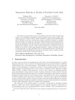
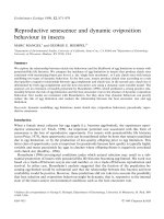
To illustrate this result, the top graph in Figure 1 plots the optimal portfolio
weight as a function of the value of the jump size m. As shown, the optimal port-
folio weight is highly sensitive to the size of the jump m.When the jump is in the

downward direction, the investor takes a smaller position in the risky asset than
he would if jumps did not occur. Surprisingly, however, the investor also takes a
smaller position when the jump is in the upward direction.The rationale for this
is related to the e¡ects of jumps on the variance and skewness of the distribution
of terminal wealth. Holding ¢xed the risk premium, jumps in either direction in-
crease the variance of the distribution. On the other hand, jumps also a¡ect the
skewness (and other higher moments) of the return distribution and the investor
bene¢ts from positive skewness. Despite this, the variance e¡ect dominates and
the investor takes a smaller position in the risky asset for nonzero values of m.The
skewness e¡ect, however, explains why the graph of f
n
against m is asymmetric.
The Journal of Finance242
To illustrate just how di¡erent portfolio choice can be in the presence of event
risk, the second graph in Figure 1plots the optimal portfolio as a function of the
risk aversion parameter g for various jump sizes m.When m 5 0 and no jumps oc-
cur, the investor takes an unboundedlylarge position in the riskyasset as g-0. In
contrast, when there is any risk of a downward jump, the optimal portfolio weight
is bounded above as g-0.This feature is a simple implication of Proposition 1, but
serves to illustrate that the optimal portfolio in the presence of event risk is qua-
litatively di¡erent from the optimal portfolio when event risk is not present.
This also makes clear that the optimal strategy is not driven purely by the
e¡ects of jumps on return skewness and kurtosis. For example, skewness and
Figure 1. Optimal portfolio weights for the constant-volatility case. The top panel
graphs the optimal portfolio weight as a function of the size of the price jump for three
di¡erent values of the jump frequency. The bottom panel graphs the optimal portfolio
weight as a function of the risk aversion coe⁄cient for three di¡erent values of the size
of the price jump.
Dynamic Asset Allocation with Event Risk 243
kurtosis e¡ects are also present in models where volatility is stochastic and cor-

related with risky asset returns, but jumps do not occur. In these models, how-
ever, investors do not place bounds on their portfolio weights of the type
described in Proposition 1. Furthermore, the optimal portfolio in these models
does not involve any static buy-and-hold component. This underscores the point
that many of the features of the optimal portfolio strategy in our framework are
uniquely related to the event risk faced by the investor.
To provide some speci¢c numerical examples,Table I reports the value of f
n
for
di¡erent values of the parameters. In this table, the risk premium for the risky
asset is held ¢xed at 7 percent and the standard deviation of the di¡usive portion
of risky asset returns is held ¢xed at 15 percent. As shown, relative to the bench-
mark where m 5 0, the optimal portfolio weight can be signi¢cantly less even
when the probability of an event occurring is extremely low. For example, even
when a À 90 percent jump occurs at a 100-year frequency, the portfolio weight is
Table I
Portfolio Weights with ConstantVolatility and Deterministic Price Jump
Sizes
This table reports the portfolio weights for the risky asset in the case where the volatility of the
asset’s returns is constant and the percentage size of the jump in the asset’s price is also con-
stant. The risk premium for the risky asset is held ¢xed at seven percent and the volatility of
di¡usive returns is held ¢xed at 15 percent throughout the table. The frequency of jumps is
expressed in years and equals the reciprocal of the jump intensity.
Risk Aversion
Parameter
Frequency of
Jumps
Percentage Jump Size
À 90 À 20 0 20 90
0.50 1 0.151 1.795 6.222 2.736 0.189

2 0.269 2.511 6.222 3.970 0.411
5 0.508 3.431 6.222 5.161 1.234
10 0.721 4.008 6.222 5.662 2.600
100 1.091 4.927 6.222 6.163 5.744
1.00 1 0.078 0.970 3.111 1.289 0.091
2 0.144 1.394 3.111 1.891 0.190
5 0.290 1.963 3.111 2.516 0.529
10 0.444 2.333 3.111 2.793 1.111
100 0.938 2.980 3.111 3.077 2.824
2.00 1 0.040 0.504 1.556 0.624 0.045
2 0.074 0.730 1.556 0.919 0.092
5 0.155 1.033 1.556 1.238 0.244
10 0.247 1.222 1.556 1.384 0.503
100 0.641 1.509 1.556 1.537 1.395
5.00 1 0.016 0.206 0.622 0.245 0.018
2 0.030 0.300 0.622 0.361 0.036
5 0.065 0.424 0.622 0.490 0.093
10 0.105 0.499 0.622 0.550 0.188
100 0.305 0.606 0.622 0.614 0.553
The Journal of Finance244
typically much less than 50 percent of what it would be without jumps. Note that
this e¡ect is not symmetric; a 190 percent jump at a 100-year frequency has a
much smaller e¡ect on the portfolio weight. Also observe that the e¡ects of jumps
on portfolio weights are much more pronounced for investors with lower levels of
risk aversion. This counterintuitive e¡ect occurs because less risk-averse inves-
tors would prefer to hold more leveraged positions, but cannot because they do
not have full control over their portfolio. Thus, the e¡ects of event risk fall much
more heavily on investors with low levels of risk aversion who would otherwise be
more aggressive.
B. StochasticVolatility and Deterministic Jump Sizes

In the second example,V is also allowed to follow a jump-di¡usion process.The
two jump sizes X andY, however, are assumed to be constants with values m and k,
respectively.The jump size m can be positive or negative.The jump size k can only
be positive.
In this example, the model dynamics become
dS
t
¼ðr þ ZV
t
À mlV
t
Þ S
t
dt þ
ffiffiffiffiffiffi
V
t
p
S
t
dZ
1t
þ mS
tÀ
dN
t
; ð26Þ
dV
t
¼ða À bV

t
À klV
t
Þ dt þ s
ffiffiffiffiffiffi
V
t
p
dZ
2t
þ kdN
t
: ð27Þ
Applying the results in Proposition 2 to this model gives the following expres-
sion for the optimal portfolio weight:
f
n
¼
Z À ml
g
þ
rsB
g
þ
lm
g
ð1 þ mf
n
Þ
Àg

e
kB
; ð28Þ
which can be solved for f
n
jointly with the equation for B given in equation (18).
Because of the dependence on B, the optimal portfolio weight is now explicitly
a function of the investor’s investment horizon. Examining equation (28) indi-
cates that there are several ways in which the investment horizon a¡ects the
optimal portfolio weight. Speci¢cally, B appears in conjunction with the correla-
tion coe⁄cient r, re£ecting that there is a dynamic hedging component to the
investor’s demand for the risky asset. SinceV is mean reverting, the horizon over
which investment decisions are made is important. However, dynamically hed-
ging shifts inV is not the only reason why there is time dependence in the optimal
portfolio weight. For example, when r 5 0, the risky asset cannot be used to hedge
against shifts in the investment opportunity set arising from variation inV.De-
spite this, the optimal portfolio weight still depends on the investor’s horizon
through the e
kB
term in equation (28).Thus, time dependence enters the problem
both through the dynamic hedging component and through the static hedging
component.
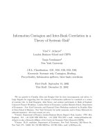
The top graph in Figure 2 plots the optimal portfolio weight as a function of the
investor’s horizon for various values of the dynamic hedging parameter r. In this
case, f
n
is an increasing function of the horizon for each of the values of r plotted.
We note, however, that f
n
can be a decreasing function of the investor’s horizon

Dynamic Asset Allocation with Event Risk 245
when go1.This graph also illustrates that the optimal portfolio weight converges
to a constant as T-N. Furthermore, the dependence of the optimal portfolio
weight on r indicates that an important part of the demand for the risky asset
comes from its ability to dynamically hedge the continuous portion of changes
inV.
An important feature of this event-risk model is that both prices and volatility
are allowed to jump. The previous section illustrated that the presence of price
jumps in either direction induces investors to take smaller positions in the risky
asset. Intuitively, one might suspect that introducing jumps in volatility would
have a similar e¡ect on the optimal portfolio weight. Surprisingly, this is not true
Figure 2. Optimal portfolio weights for the stochastic-volatility case. The top panel
graphs the optimal portfolio weight as a function of the investor’s horizon measured in
years for three di¡erent values of the correlation coe⁄cient. The bottom panel graphs
the optimal portfolio weight as a function of the size of the volatility jumps for three dif-
ferent values of the size of the price jump.
The Journal of Finance246
in general. This can be seen from the second graph in Figure 2, which plots the
optimal portfolio weight as a function of the size of the volatility jump k for dif-
ferent values of m. As shown, the optimal portfolio weight can be an increasing
function of k for some values of m.
This result illustrates the important point that in addition to its ability to dy-
namically hedge against continuous changes inV, the risky asset can alsobe used
as a static hedge against the e¡ects of jumps inV.This second hedging role is one
that does not occur in traditional portfolio choice models where state variables
have continuous sample paths.The fact that the risky asset can be used to hedge
in two di¡erent ways, however, makes it evident that the investor faces a dilemma
in choosing a portfolio strategy. In particular, the portfolio that hedges against
small local di¡usion-induced changes in the state variables is not the same as the
portfolio that hedges against large jumps in the state variables. This problem is

inherent in the fact that when there is event risk, the portfolio problem has fea-
tures of both a dynamic portfolio problem and an illiquid buy-and-hold problem.
Finally, if we impose the parameter restrictions r 5 0andk 5 0, volatility is
still stochastic, but the optimal portfolio weight becomes the same as in Section
III.Awhere volatility is not stochastic.Thus, continuous stochastic variation inV
only a¡ects the optimal portfolio weight if it is hedgable through a nonzero value
of r.
IV. Implications for Optimal Portfolio Choice
Moving beyond the numerical examples presented in Section III, it is useful to
explore how event risk might a¡ect the optimal portfolio of an investor in a spe-
ci¢c market. To this end, we calibrate the model to be roughly consistent with
historical stock index returns and stock index return volatility in the United
States.To make this process as straightforward as possible, we focus on the sim-
ple stochastic volatility model with deterministic jump sizes described in Section
III. Once calibrated to U.S. data, we explore the key implications of the model for
investors.
In parameterizing this model of event risk, it is important to recognize that the
major ¢nancial events addressed by our model are infrequent by their nature. Ide-
ally, we would like to use a calibration approach that minimizes the e¡ects of the
inherent ‘‘Peso problem’’on the results. Although there are many ways to do this,
we use the following informal (but, we hope, intuitive) approach to allow us to
estimate the size and frequency of events from the longest time series available.
10
We ¢rst obtain the monthly return series for U.S. stocks during the 1802 to 1925
period created and described in Schwert (1990). We then append the CRSP
monthly value-weighted index returns for the 1926 to 2000 period to give a time
series of returns spanning nearly 200 years. A review of the data shows that there
10
We note that although it is beyond the scope of this paper, the general double-jump model
could be formally estimated using either the e⁄cient method of moments (EMM) approach

applied by Andersen, Benzoni, and Lund (2002) or the Monte Carlo Markov chain (MCMC)
technique used by Eraker et al. (2000).
Dynamic Asset Allocation with Event Risk 247
are eight observations where the stock index dropped by 20 percent or more.
These observations include the beginning of the Civil War in May 1861, the black
Friday crash of October 1929, and the October 1987 stock market crash. Interest-
ingly, four of the eight observations are clustered in the high-volatility decade of
the 1930s, consistent with the double-jump model. Since these observations are
roughly ¢ve standard deviations below the mean, it is not unreasonable to view
these negative returns as being due to ajump event. A back-of-the-envelope calcu-
lation suggests calibrating the model to allow a À 25 percent jump (the average of
the eight observations) at an average frequency of about 25 years. To provide a
rough estimate of the size of the volatility jump, we compute the standard devia-
tion of returns for the ¢ve-month window centered at the event month. The aver-
age of these standard deviation estimates is just under 50 percent. Given this, we
make the simplifying assumption that when a jump occurs, the volatility of the
stock return jumps by an amount equal to the di¡erence between 50 percent and
its mean value.
The remaining parameter estimates are obtained from Table 1 of Pan (2002).
Using S&P 500 stock index returns and stock index option prices, Pan estimates
the parameters of several versions of a jump-di¡usion model. For simplicity, we
use the parameter values Pan estimates for her SV0 model, and adjust them
slightly to be consistent with our estimates of jump sizes and frequencies.
11
Spe-
ci¢cally, we use Pan’s estimates of b 5 5.3 and r 5 À .57.To obtain estimates of a, Z,
and s, we note that in our model, the expected instantaneous equity premium is
aZ/b, the expected instantaneous variance of returns is a(11m
2
l)/b, and the ex-

pected instantaneous variance of changes inV is a(s
2
1k
2
l)/b. Setting these three
moments equal to the corresponding estimates of 0.1065, 0.0242, and 0.3800 from
Table 1of Pan provides us with three equations which can be solved for the values
of a, Z,ands. By doing this, we guarantee that the calibrated model matches the
moments of returns and volatility estimated by Pan. This approach leads to the
following parameter values for the baseline case where jumps occur with an
average frequency of 25 years: a 5 0.11512, b 5 5.3000, s 5 0.22478, Z 5 4.90224,
r 5 À 0.57000, m 5 À 0.25000, k 5 0.22578, and l 5 1.84156.
To illustrate the e¡ects that event risk has on the optimal portfolio choice for an
investor where the model is calibrated to historical U.S. returns in this manner,
Table II reports the portfolio weights for various levels of investor risk aversion.
To facilitate comparison, we report the portfolio weights for the case where there
are no jumps, where there are only jumps in the stock index, and the baseline case
where there are jumps in both the stock index and volatility. Note that for the non-
benchmark cases, we recalibrate the model so that we match the expected instan-
taneous moments estimated by Pan (2002) using the procedure described in the
previous paragraph. In each case, the investor has a ¢ve-year investment horizon.
11
The advantage of using the parameter estimates for Pan’s SV0 model is that they repre-
sent parameter estimates for the stochastic volatility model in the absence of jumps.This then
allows us to calibrate the model for di¡erent jump sizes using a particularly simple algorithm.
As pointed out by Pan, allowing for jumps signi¢cantly enhances the ability of the stochastic
volatility model to capture the properties of the data.
The Journal of Finance248
Table II shows that the possibility of a 25 percent downward jump in stock
prices has an important e¡ect on the investor’s optimal portfolio, even though

this type of event happens only every 25 years on average. For example, the opti-
mal portfolio weight for an investor with a risk aversion parameter of two is 2.305
if no jumps can occur, is 1.929 if only jumps in the stock price can occur, and is
2.010 if both jumps in stock prices and volatility can occur. Observe that from
Proposition 1, the investor never takes a position in the risky asset greater than
four since jumps of À 25 percent can occur.Table II shows that the risk of a down-
ward jump always induces the investor to take a smaller position in the stock
market than he would otherwise.
Table II also makes clear that while jumps in volatility do not have as much of
an e¡ect as jumps in the stock price, they do have an important in£uence on the
optimal portfolio. Interestingly, jumps involatility decrease the optimal portfolio
weight when go1, and increase the optimal portfolio weight when g41. Intui-
tively, the reason for this is related to the e¡ect of a volatility jump on the distri-
bution of the investor’s returns. Recall that in this model, the instantaneous
Sharpe ratio of returns is increasing in the volatility V because of the form of
the risk premium.Thus, when an event occurs, the investor su¡ers an immediate
loss because of the downward jump in the stock price, but then faces an improved
Table II
Portfolio Weight and Wealth Equivalent Loss Comparisons for the Cali-
brated Model Where Jumps Occur Every 25 Years on Average
This table reports portfolio weights for the stochastic volatility model with deterministic jumps
in prices and volatility. Also reported are the percentage wealth equivalent losses for an inves-
tor who ignores the possibility of event-related jumps.This loss re£ects the cost (as a percentage
of his wealth) to an investor who assumes that jumps cannot occur, calibrates the model to
match historical moments, and follows the portfolio strategy he believes is optimal, but is actu-
ally suboptimal in cases where jumps can occur.The average frequency of an event is 25 years.
The ¢rst column reports the portfolio weights when the jump sizes are both zero (no jumps).The
second column reports the portfolio weights and wealth equivalent losses when the stock price
jump is À 25 percent and the volatility jump is zero (stock jumps only).Thethird column reports
the portfolio weights and wealth equivalent losses for the baseline case where the stock price

jump is À 25 percent and the volatility jumps to 50 percent. Each scenario is calibrated to match
the parameter estimates inTable 1 of Pan (2002).
No Jumps Stocks Jumps Only
Both Stock and Volatility
Jumps
Risk Aversion
Parameter
Portfolio
We ight
Portfolio
We i g h t
Wealth
Equivalent
Loss
Portfolio
We i g h t
Wealth
Equivalent
Loss
0.50 8.106 3.914 100.0 3.865 100.0
1.00 4.396 3.163 100.0 3.163 100.0
2.00 2.305 1.929 3.2 2.010 2.0
3.00 1.564 1.356 1.3 1.432 0.5
4.00 1.183 1.042 0.7 1.107 0.2
5.00 0.952 0.845 0.5 0.901 0.1
Dynamic Asset Allocation with Event Risk 249
risk-return trade-o¡ because the jump in volatility increases the Sharpe ratio.
This pattern induces a type of negative serial correlation or smoothness into
the time series of the investor’s returns which can be shown to reduce both the
¢rst and second moments of the distribution of the investor’s terminal wealth. As

shown by Samuelson (1991), however, investors who are less risk averse than loga-
rithmic (go1), will reduce their portfolio weight as this smoothing increases,
while the opposite is true for investors who are more risk averse than logarith-
mic.Thus, an increase in the volatility jump size parameter k leads to a decrease
in the portfolio weight for go1, and to an increase in the portfolio weight for g41.
Another way of seeing this is to note that for g41, the investor’s utility is un-
bounded from below as his wealth approaches zero.Thus, the investor is particu-
larly averse to a run of successive negative returns. Since a jump inVreduces the
likelihood of a run of negative returns, the investor with g41 is more con¢dent
and takes a larger stock position. In contrast, for go1, the investor’s utility is
bounded from below but unbounded from above. Thus, the investor bene¢ts less
from the reduction in variance of the distribution of terminal wealth and reduces
his portfolio weight because of the reduction in the ¢rst moment.
12
Another interesting issue to consider is the loss su¡ered by an investor who
does not consider the e¡ects of price and volatility jumps in making portfolio
decisions.
13
To examine this, we do the following. Assume that there is an investor
who believes that there are no jumps, implying that l 5 m 5 k 5 0. This investor
calibrates his model to match the moments using the procedure described ear-
lier. Given this calibration, the investor then follows the portfolio strategy that
would be optimal if l 5 m 5 k 5 0. Let us denote this strategy
^
ff. Now assume that
there are actually jumps in prices and volatility. In this situation, the optimal
portfolio weight f
n
di¡ers from
^

ff, and the investor su¡ers a loss by following this
strategy. Following a procedure similar to that used to solve for J(W,V, t), we can
solve for the investor’s utility of wealth function when he follows strategy
^
ff.De-
note this utility of wealth function K(W,V, t). Because
^
ff is suboptimal, it is clear
that K(W, V, t)oJ(W, V, t). To quantify the loss, we assume that this investor
following the suboptimal strategy starts withW 5 1, and solve for the
^
WW suchthat
an investor with W ¼
^
WW who followed the optimal strategy would attain the
same level of utility. Speci¢cally, this utility equivalent wealth
^
WW is obtained by
solving numerically the equation Jð
^
WW; V; tÞ¼Kð1; V; tÞ. Note that the utility
equivalent wealth
^
WW is less than or equal to one since following the suboptimal
strategy
^
ff reduces the utility of the investor’s wealth. Finally, we calculate the
loss using this wealth-based metric by taking the di¡erence 1 À
^
WW and convert-

ing it into percentage terms by multiplying by 100. We designate this metric the
wealth equivalent loss.
Table II reports the wealth equivalent losses for an investor who does not con-
sider the e¡ects of jumps.There are several key features shown in Table II. First,
12
Consistent with this intuition, when both stock price and volatility jumps are positive,
the e¡ect of an increase in the volatility jump size parameter k is reversed. In particular,
the portfolio weight is then an increasing function of k for go1, and vice versa.
13
We are grateful to the referee for raising this issue.
The Journal of Finance250
when the suboptimal strategy
^
ff exceeds the bound in Proposition 1, then a jump
to ruin is possible and clearly, K(W,V, t) 5 À N. In these cases, it is clear that the
wealth equivalent loss of following the suboptimal strategy is 100 percent; the
investor obtains the same expected utility that he would if he had no wealth at
all. Second, Table II shows that the wealth equivalent loss can be nontrivial for
other ranges of the risk aversion parameter. Speci¢cally, when g 5 2.00, the
wealth equivalent loss is 3.2 percent when only price jumps can occur, and is 2.0
percent when both price and volatility jumps can occur.Table II also shows that
the wealth equivalent loss is a decreasing function of g.
Although we have calibrated the model to historical U.S. returns, it is impor-
tant to recognize that U.S. returns may not fully re£ect the size of potential jump
events. The reason for this is the possibility of a survivorship bias, since the
United States has experienced historically high returns.This point is alsoconsis-
tent with Jorion and Goetzmann (1999) who show that many countries have ex-
perienced huge market declines during relatively short periods of time during
the past century. In many cases, major events such as wars or political crises have
actually led to stock markets being closed for years (or even decades). These

closures have often resulted in catastrophic losses for investors. To re£ect this
downside risk to ¢nancial markets, we also consider a scenario where stock mar-
ket jumps of À 50 percent and volatility jumps to 70 percent occur at an average
frequencyof100 years. Following the same calibration approach as before implies
parameter values for this scenario of a 5 0.11512, b 5 5.3000, s 5 0.21099,
Z 5 4.90224, r 5 À 0.57000, m 5 À0.50000, k 5 0.46578, and l 5 0.46039.
Table III reports the optimal portfolio weights for this alternative scenario.
Even though the frequency of an event is much less, it has an even larger e¡ect
on the optimal portfolio weight than in Table II. For example, the optimal portfo-
lio weight for an investor with a risk aversion parameter of two is still 2.305 if no
jumps can occur. If only jumps in the stock price can occur, then the portfolio
weight is now 1.395 rather than 1.929. If both jumps in the stock price and volati-
lity can occur, the optimal portfolio weight is now 1.481 rather than the value of
2.010 given in Table II. As before, jumps in volatility decrease the optimal portfo-
lio weight for go1, and vice versa.
Table III also reports the corresponding wealth equivalent losses. As in Table
II, the wealth equivalent loss can be 100.0 percent when the bound given in Pro-
position 1 is violated. It is interesting to note, however, that there is a case shown
in Table III where an investor following the suboptimal strategy attains K(W,V,
t) 5 À N even when
^
ff does not violate the bound given Proposition 1. Speci¢-
cally, when g 5 3.00, an investor who does not consider the e¡ects of volatility
jumps has a portfolio weight of 1.564 (which does not violate the bound) but still
has a wealth equivalent loss of 100.0 percent when both price and volatility jumps
can occur. Intuitively, this occurs because the ¢niteness of the expected utility
function can only be guaranteed when the optimal strategy f
n
is followed.
14

Spe-
ci¢cally, when the suboptimal portfolio weight
^
ff is su⁄ciently high (but still less
than the bound given in Proposition 1), the return distribution for the investor’s
14
Note that in this case, g 5 3, which means that utility is unbounded from below.
Dynamic Asset Allocation with Event Risk 251
wealth may be such that the expectation of his terminal utility equals À N.For
example, consider the case where g 5 2, and expected utility equals À E[1/W
T
].
Even though all positive moments of the distribution of W
T
are ¢nite when
^
ff is
followed, the expectation E[1/W
T
}] may fail to exist, implying K(W,V, t) 5 À N.
Thus, even when a jump to complete ruin cannot occur, a strategy may be so sub-
optimal that the investor has a wealth equivalent loss of 100 percent.
15
Another
way of seeing this is by considering the case where the stock price jump is À 50
percent. By following a strategy where f is less than two, ruin can be avoided.
However, imagine that
^
ff is close to two, say 1.99. If a jump occurs, the investor
will clearly lose virtually all of his wealth. After the jump, however, the investor

would rebalance his portfolio to attain
^
ff ¼ 1:99 again.Thus, if another jump oc-
curs, the investor’s remaining wealth will again be virtually eliminated.The key
point is that even though total ruin does not occur, the resulting distribution of
W
T
has enough mass in the neighborhood of zero that the expected utility func-
tion need not be ¢nite.When f is more distant from the bound in Proposition 1, as
is the case for f
n
, this situation does not arise and expected utility is ¢nite.
Table III
Portfolio Weight and Wealth Equivalent Loss Comparisions for the Cali-
brated Model Where Jumps Occur Every 100 Years on Average
This table reports portfolio weights for the stochastic volatility model with deterministic jumps
in prices and volatility. Also reported are the percentage wealth equivalent losses for an inves-
tor who ignores the possibility of event-related jumps.This loss re£ects the cost (as a percentage
of his wealth) to an investor who assumes that jumps cannot occur, calibrates the model to
match historical moments, and follows the portfolio strategy he believes is optimal, but is actu-
ally suboptimal in cases where jumps can occur.The average frequency of an event is 100 years.
The ¢rst column reports the portfolio weights when the jump sizes are both zero (no jumps).The
second column reports the portfolio weights and wealth equivalent losses when the stock price
jump is À 50 percent and the volatility jump is zero (stock jumps only). The third column re-
ports the portfolio weights and wealth equivalent losses for the baseline case where the stock
price jump is À 50 percent and the volatility jumps to 70 percent. Each scenario is calibrated to
match the parameter estimates in Table 1 of Pan (2002).
No Jumps Stocks Jumps Only
Both Stock and Volatility
Jumps

Risk Aversion
Parameter
Portfolio
We ight
Portfolio
We i g h t
Wealth
Equivalent
Loss
Portfolio
We i g h t
Wealth
Equivalent
Loss
0.50 8.106 1.993 100.0 1.987 100.0
1.00 4.396 1.859 100.0 1.859 100.0
2.00 2.305 1.395 100.0 1.481 100.0
3.00 1.564 1.059 30.5 1.174 100.0
4.00 1.183 0.844 11.2 0.956 5.3
5.00 0.952 0.698 6.3 0.801 2.2
15
This feature appears in many other continuous time portfolio choice models and is not
unique to jump di¡usion models. For other examples, see Liu (1999).
The Journal of Finance252
Finally,Table III shows the wealth equivalent losses can be signi¢cant for other
parameter values. For example, when only price jumps can occur, an investor
with g 5 3.00 who ignores the e¡ects of jumps has a wealth equivalent loss of
30.5 percent. For larger values of g, the wealth equivalent losses are smaller, but
are still economically signi¢cant.
The results inTables II and III are based on two simple calibrations of the mod-

el. Given than there is always uncertainty about the precise values of estimated
parameters, however, it is useful to provide some additional information about
the sensitivity of the optimal portfolio weights to the key jump size and frequency
parameters.To this end,Table IVreports the optimal portfolio weights for various
combinations of jump frequencies and price jump sizes, while TableVreports the
optimal portfolio weights for various combinations of jump frequencies and vola-
tility jump sizes. For each set of jump size and frequency parameters in these two
tables, the a, Z,ands parameters are chosen to match the three moments from
Table 1 of Pan (2002) using the same procedure as before. We note that in a few
cases involving large but infrequent jumps, these moments cannot be matched,
since they imply negative values for s; these cases are designated by a dash in
Tables IVand V.
Tables IVand V indicate that the optimal portfolio weight is clearly a¡ected by
both the jump size and frequency parameters.The size of the price jump appears
to have the largest e¡ect on the optimal portfolio weight.The size of the volatility
jump as well as the level of the frequency parameter can also have important ef-
fects. Despite this dependence on the parameter values, however,Tables IVand V
indicate that the optimal portfolio weight is generally fairly robust to small per-
turbations in the parameter values.This is important, since it implies that even if
the jump size and frequency parameters are estimated with some error (provided
it is not overly large) from historical data, the general implications for optimal
portfolio choice may still be qualitatively valid.
Admittedly, we have focused only on simple calibrations of one of the simplest
versions of the model. Despite this, however, we believe that several important
general insights about the role that event risk could play in real-world portfolio
decisions emerge from this analysis. Foremost among these is that investors have
strong incentives to signi¢cantly reduce their exposure to the stock market when
they believe that there is event risk. This is true even when the probability of a
major downward jump in stock prices is very small, as in the scenario of a À 50
percent jump occurring every 100 years on average. Certainly, jumps of this mag-

nitude and frequency cannot be ruled out; it is all too easy to think of extreme
situations where a downward jump of this magnitude could occur during the
next century even in the United States, particularly in the wake of September
11, 2001. Our analysis suggests a possible reason why historical levels of partici-
pation in the stock market have been much lower than standard portfolio choice
models would view as optimal.
16
16
For example, see Mankiw and Zeldes (1991), Heaton and Lucas (1997), and Basak and Cuo-
co (1998).
Dynamic Asset Allocation with Event Risk 253
V. C o n c l u s i on
In this paper, we study the e¡ects of event-related jumps in prices and volatility
on investment strategies. Using the double-jump framework of Du⁄e et al. (2000),
we take advantage of the a⁄ne structure of the model to provide analytical solu-
tions to the optimal portfolio problem.
Table IV
Portfolio Weights for the Calibrated Model for Varying Percentage Price
Jumps and Jump Frequencies
This table reports portfolio weights for the stochastic volatility model with deterministic jump
sizes in prices and volatility. Each combination of parameters is calibrated to match the para-
meter estimates inTable 1of Pan (2002).The frequency of jumps is expressed in years and equals
the reciprocal of the jump intensity. Sets of parameters for which the moments cannot be
matched are denoted by a dash.
Risk
Aversion
Parameter
Volatility
Jumps to
Frequency

of Jumps
Percentage Price Jump Size
À 10 À20 À 30 À 40 À 50
0.50 25 20 7.772 4.825 3.219 2.398 1.900
30 7.871 4.903 3.272 2.444 1.945
40 7.924 4.938 3.295 2.465 1.965
50 7.958 4.957 3.307 2.476 1.976
100 8.029 4.987 3.326 2.493 1.993
0.50 50 20 7.757 4.752 3.175 FF
30 7.838 4.855 3.246 2.423 1.925
40 7.892 4.906 3.278 2.452 1.953
50 7.929 4.934 3.295 2.467 1.968
100 8.011 4.979 3.322 2.490 1.991
2.00 25 20 2.287 2.091 1.687 1.325 1.066
30 2.293 2.149 1.790 1.426 1.153
40 2.296 2.182 1.858 1.496 1.216
50 2.298 2.204 1.908 1.549 1.264
100 2.302 2.251 2.040 1.702 1.403
2.00 50 20 2.262 2.130 1.764 FF
30 2.281 2.184 1.859 1.494 1.217
40 2.288 2.211 1.920 1.557 1.270
50 2.292 2.228 1.964 1.605 1.312
100 2.299 2.265 2.081 1.746 1.440
5.00 25 20 0.948 0.897 0.776 0.639 0.528
30 0.949 0.913 0.814 0.686 0.572
40 0.950 0.922 0.839 0.719 0.605
50 0.950 0.928 0.855 0.743 0.631
100 0.951 0.939 0.896 0.811 0.708
5.00 50 20 0.928 0.917 0.839 FF
30 0.939 0.931 0.870 0.762 0.655

40 0.943 0.937 0.885 0.784 0.674
50 0.945 0.940 0.895 0.801 0.693
100 0.949 0.946 0.920 0.852 0.755
The Journal of Finance254
The presence of event risk changes the standard portfolio problem in several
important ways. First, since the investor no longer has complete control over his
wealth, the investor acts as if some part of his portfolio consists of illiquid assets
and he is much less willing to take leveraged or short positions.The optimal port-
folio strategy blends elements of both a standard dynamic hedging strategy and a
buy-and-hold or ‘‘illiquidity’’ hedging strategy. Furthermore, event risk a¡ects
TableV
Portfolio Weights for the Calibrated Model for Varying Volatility Jump
Sizes and Jump Frequencies
This table reports portfolio weights for the stochastic volatility model with deterministic jump
sizes in prices and volatility. Each combination of parameters is calibrated to match the para-
meter estimates in Table 1of Pan (2002).The frequency of jumps is expressed in years and equals
the reciprocal of the jump intensity. Sets of parameters for which moments cannot be matched
are denoted by a dash.
Risk Aversion
Parameter
Percentage
Price Jump
Frequency
of Jumps
Volatility Jumps to
20 30 40 50
0.50 À 25 20 3.876 3.861 3.841 3.816
30 3.932 3.924 3.912 3.896
40 3.958 3.953 3.945 3.934
50 3.971 3.967 3.962 3.954

100 3.992 3.991 3.989 3.986
0.50 À 50 20 1.905 1.894 1.877 F
30 1.947 1.942 1.935 1.925
40 1.966 1.964 1.959 1.953
50 1.977 1.975 1.972 1.968
100 1.993 1.993 1.992 1.991
2.00 À25 20 1.885 1.911 1.942 1.963
30 1.976 1.996 2.022 2.044
40 2.033 2.050 2.071 2.091
50 2.072 2.087 2.105 2.123
100 2.167 2.177 2.188 2.199
2.00 À50 20 1.054 1.080 1.117 F
30 1.146 1.163 1.188 1.217
40 1.209 1.224 1.245 1.270
50 1.258 1.271 1.289 1.312
100 1.399 1.409 1.423 1.440
5.00 À 25 20 0.833 0.854 0.878 0.887
30 0.864 0.880 0.897 0.090
40 0.882 0.894 0.908 0.918
50 0.894 0.904 0.916 0.924
100 0.920 0.926 0.932 0.937
5.00 À 50 20 0.515 0.546 0.596 F
30 0.562 0.584 0.616 0.655
40 0.597 0.615 0.641 0.674
50 0.623 0.640 0.663 0.693
100 0.702 0.715 0.733 0.754
Dynamic Asset Allocation with Event Risk 255